Trading the mean reversion curve

A portfolio of mean-reversion strategies that delivers 26% annual returns since 2010

Jul 27, 2024

James Joyce bust in Kielce, Poland. Joyce is regarded as one of the most influential writers of the 20th century.

The idea

"Mistakes are the portals of discovery." James Joyce.

I think this is my best post so far. It's not because of any particular great results (although they are nice). It's because I got help from three extraordinary people: a Market Wizard and a couple of traders who talked about mean reversion in one of the top podcasts for systematic traders. Curiously, it all started with an error.

Hours after I published the last article, I received a kind email from Marsten Parker. Some weeks ago, I wrote an implementation about his IPO strategy. He is best known for being featured in Jack Schwager's book Unknown Market Wizards, where he is highlighted as the only purely systematic trader in the series.

He implemented the strategy I had just published in RealTest, his amazing backtesting software, and wrote: “My results were similar, but different enough to be worth asking you about.” The email described what could be causing the differences (there are many, many little details in the backtest logic that can lead to divergences). Additionally, he was kind enough to share the trade list output from the backtest, which was crucial to debugging.

Comparing his trades to mine, I found something funny: several trades were the same, but some were missing on my side. Digging into the differences, I found a problem on my side with data conversion from one system to another. Here’s what the issue was:

I use a MacBook Pro M3 (Apple Silicon OS) and don’t have access to a Windows machine.
To use Norgate Data, the new dataset I acquired a few days ago, I had to install Windows in a Virtual machine (UTM), extract the data there using Python, share the file between systems, and get it on the MacOS to run my analysis.
Something got lost in this conversion (I can’t explain exactly why, but I’ve seen something similar when running PyTorch/GPU code).
Strangely, when I computed RSI2 and NATR using Talib (a C++ technical analysis library) on the file extracted from Windows, about ~20% of the values became NaNs, which completely messed up with the numbers.

The solution was as simple as using another format to save the data and transfer the file from one system to another. Re-running all the tests, we came to the same results.

Again, I would like to thank Marsten for his help in debugging and improving this system. Systematic trading is hard, and even if we take all precautions, some unimaginable errors might occur. Moreover, I believe openly discussing trading systems and ideas can help us prevent those errors and become better at the craft. Mistakes, after all, are the portals of discovery.

Talking about discovery, one of the things I discovered because of the error was his RealTest backtesting software. It's a fantastic system. All results presented here were double-checked with RealTest (excluding the diversification algorithm).

The plan for this article is:

First, I will recompute the edge and the best experiment from the last article, discussing the differences;
Then, I will iterate through key parameters, improving the system;
Next, I will introduce the idea of trading the mean reversion curve, creating a portfolio of mean reversion strategies to improve the performance in recent history;
Finally, I will re-do the slippage and trading costs analysis.

The edge

Let's recompute the edge of buying the stocks whenever their 2-period RSI closes below 5 (and the stock price is above its 200-day SMA) and holding them for a few days.

We will do something different, though: compute it for different thresholds (not only 5). We start with 5:

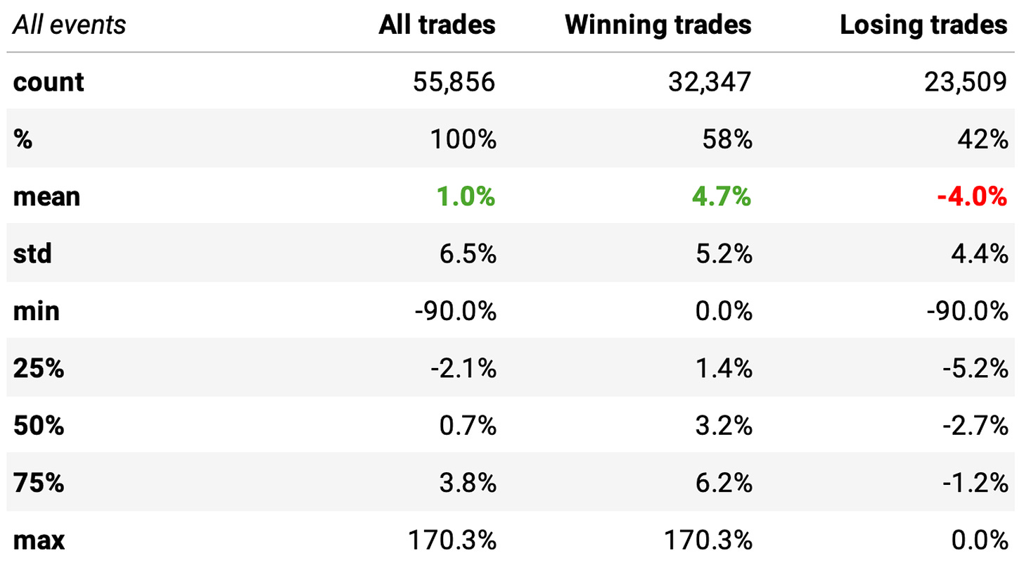
Statistics of buying Nasdaq-100 constituents when 2-day RSI closes below 5 and holding for 5 days, recomputed

Although the numbers are slightly different than what we obtained in the other article, the conclusions are the same:

The win rate is 58%, much better than a coin-flip;
There is a positive payoff ratio: winning trades are expected to generate +4.7% while losing trades -4.0% (4.7/4.0 > 1);

The statistics of the non-events are precisely the same as those obtained previously (I won't repeat them; you can check them here). Also, the P-value continues well below 0.05: the means of the two distributions are significantly different. So, we have an edge.

Frequency of entry triggers

One thing that I didn't include in the previous article was the frequency of events. On average, how many stocks trigger the entry rule (RSI2 < 5) on a given day? Here's the data:

Frequency of events (63-day MA to smooth the curve). The median value is 4.

As we can see, the number of stocks triggering the entry rule oscillates around the 4 median value. This number will be important when we choose the maximum number of positions to hold at any given time.

The impact of volatility

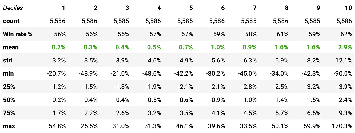
Let's recompute how this edge varies with respect to volatility, measured as (normalized) Average True Range.

Impact of the NATR on the Expected Return

Again, the conclusion is the same: the higher the volatility, the higher the expected return in these short-term mean-reversion trades.

However, the figures are much better than what I had previously assessed. The expected return gain from stocks with high volatility is way higher than what we computed in the last article.

The impact of the entry threshold

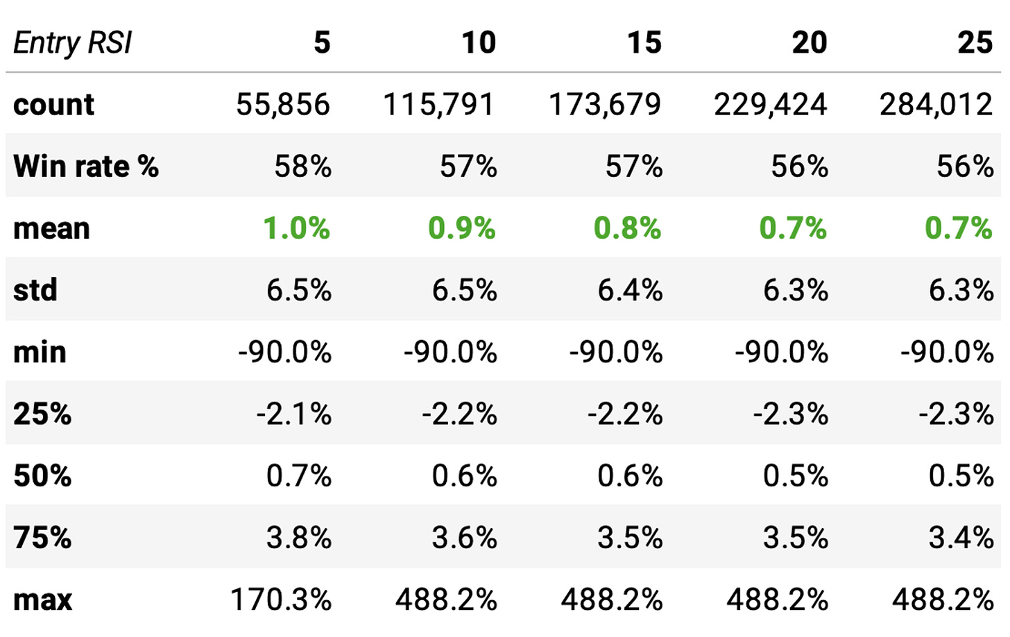
This session is new compared to the last article. The reason to include it will be revealed soon. We are trying to answer the question: how does the RSI2 entry threshold level impact the edge? Here's the answer:

Impact of the Entry RSI threshold on the expected return

We can draw two important conclusions from the data above:

First, as we tighten the threshold to enter trades, reducing the maximum RSI2 value, we increase the edge: the expected return increases, as well as the win rate. Conversely, as we relax the threshold, increasing the maximum RSI2 value, the edge decreases: the expected return diminishes, and the win rate drops. This is because a tighter threshold ensures that trades are only entered under more favorable conditions, thereby increasing the likelihood of success. On the other hand, a looser threshold allows for trades under less favorable conditions, which can lead to a higher number of trades but with reduced overall profitability and a lower win rate.
Although looser thresholds show lower expected returns, they offer more opportunities to trade: the number of stocks triggering the entry rule is higher. This might be beneficial to increase exposure in market conditions when there are not enough strong signals from tighter thresholds. In such scenarios, loosening the thresholds can help ensure the portfolio remains active and engaged in the market.

The strategy

We will start with the same strategy we used in the last article:

At the opening of every trading session:

We will split our capital into 10 slots and buy stocks whose 2-day RSI from the previous day closed below 5;
If there are more than 10 stocks in the universe with the entry signal triggered, we will sort them by Normalized Average True Range and prioritize the high-volatility stocks;
We will hold 10 positions maximum at any given moment;
When the stock closes above yesterday's high, we will exit on the next open;
We will only trade Nasdaq-100 constituents (at the specific past date).

Experiments

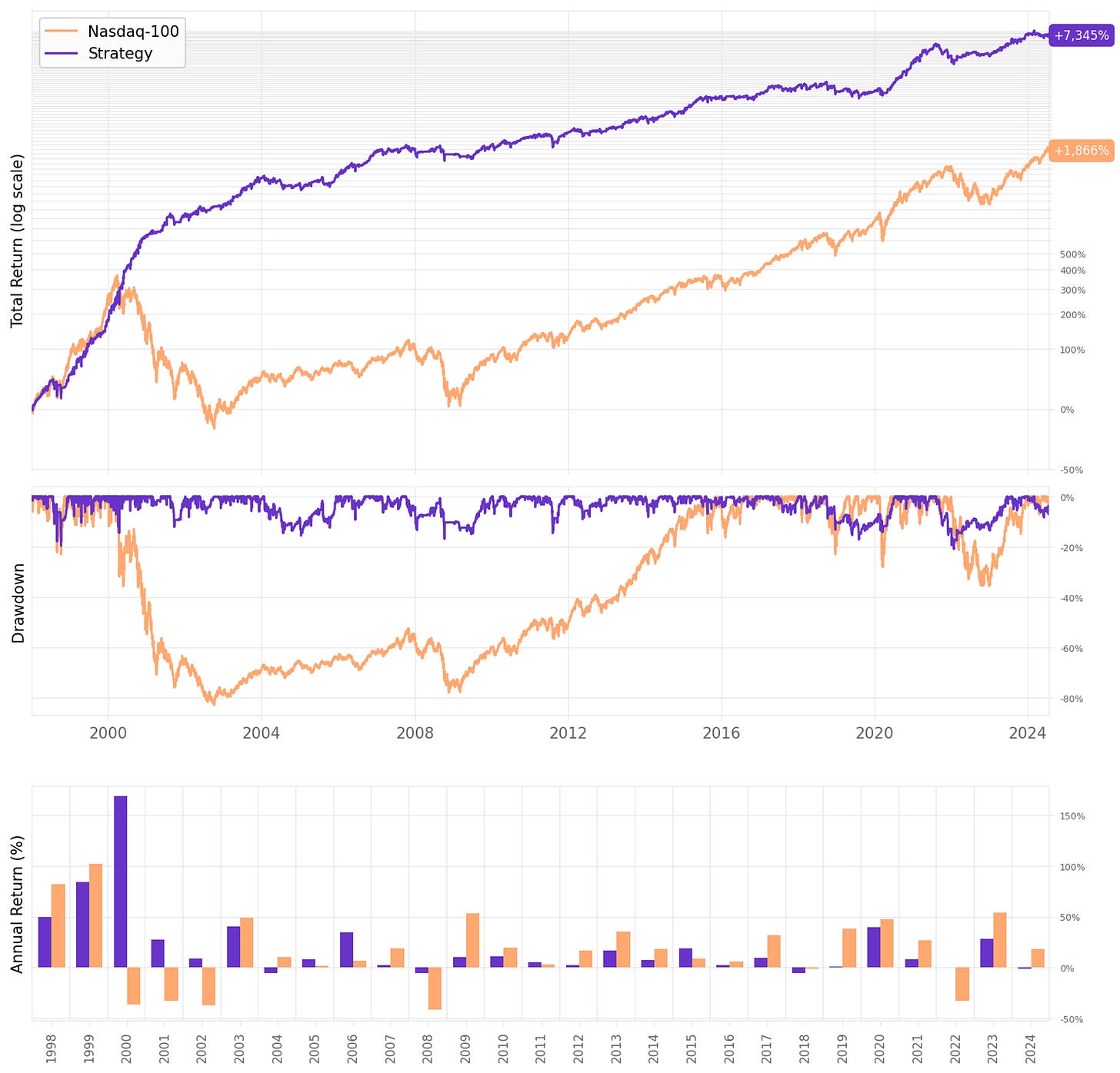
Here are the first results to contrast with what we achieved earlier:

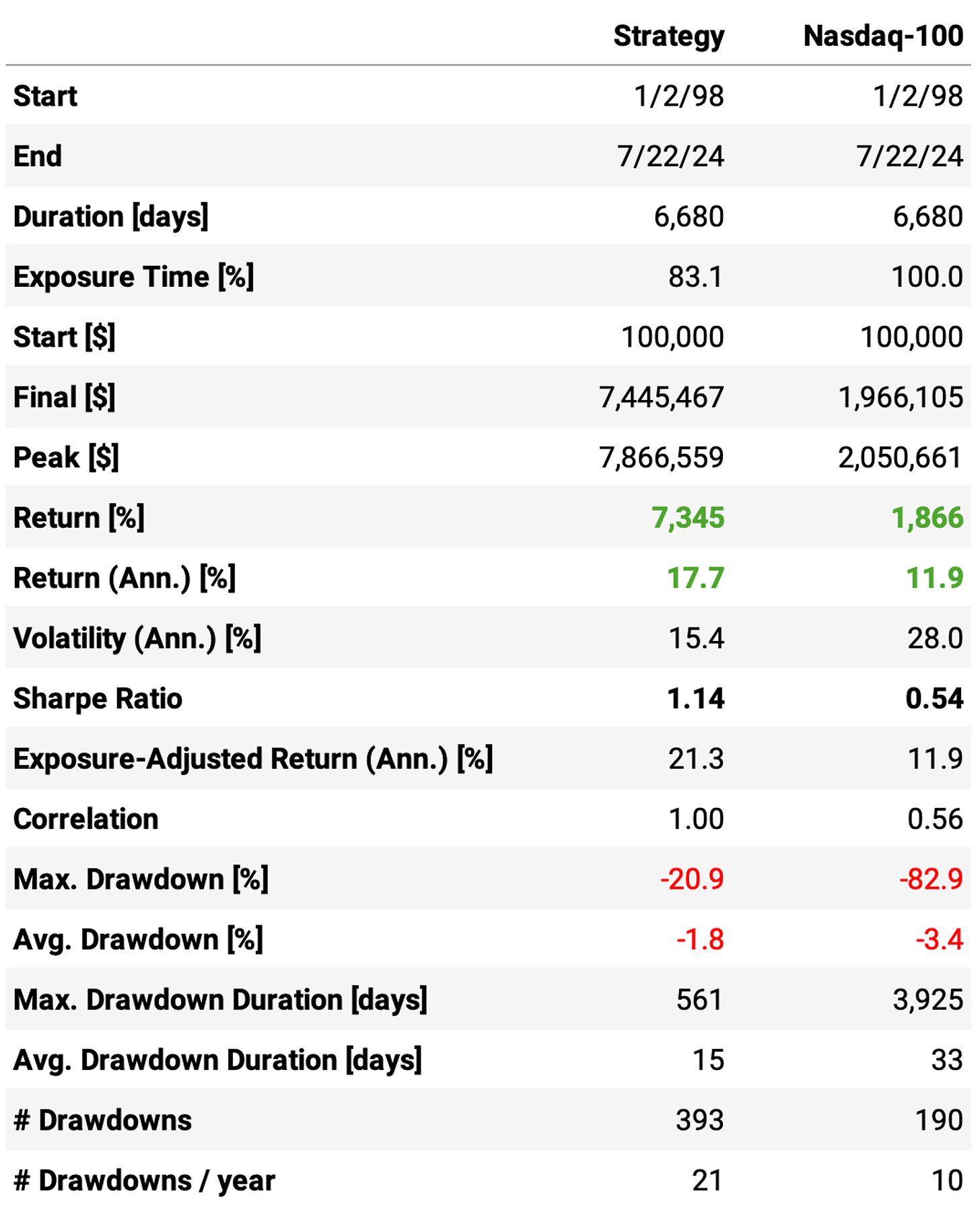
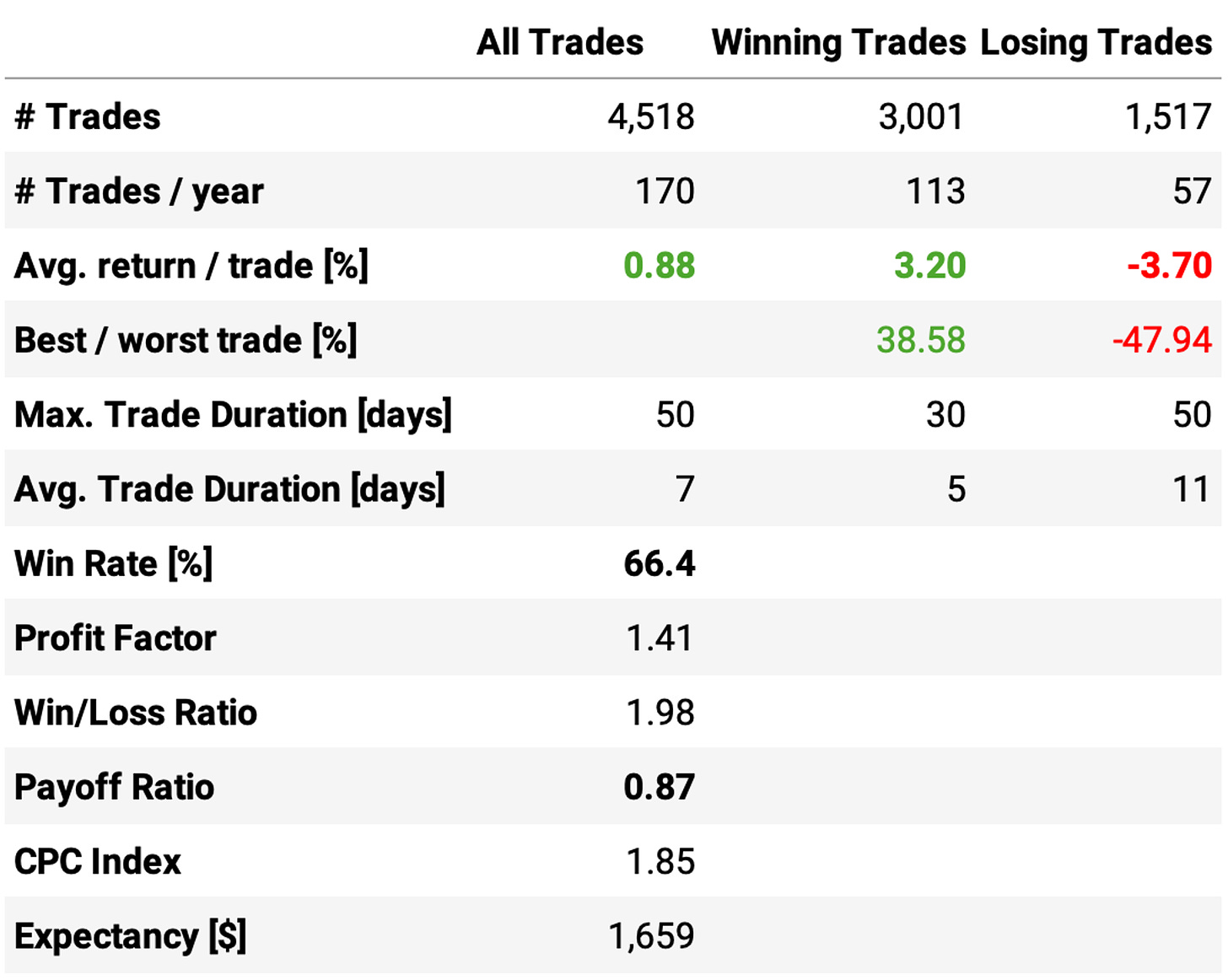
Equity and drawdown curves for the first experiment

Fixing the data conversion error led to different results. As Marsten said, “similar but different enough to be noted.” Here are the highlights:

Instead of 23% annual returns, we achieved 18% annual returns. It's still above the benchmark (12%), but not as much;
The maximum drawdown is significantly better at 21% instead of the 34% we saw in the previous article;
Lower drawdowns, lower volatility, and better risk-adjusted return: now, we achieved a 1.14 Sharpe vs. 0.98 seen previously;
Also, all the trade statistics are better: higher win rate, profit factor, and payoff ratio.

However, it's important to observe two facts:

First, the strategy lost steam from 2008 on. Apparently, all the best years were two decades ago, between 2000 and 2010. This is not good.
Second, the exposure time is significantly lower, now at 83% (instead of the 99% we saw in the previous article). Apparently, the data conversion issue led the system to trigger lower-quality entries more often. With the problem fixed, we have better trades but fewer trades. In fact, when we look at the average number of trades per year, we see a sizable reduction from 221/year to 170/year.

How can we improve the system?

Loosening the RSI2 entry threshold

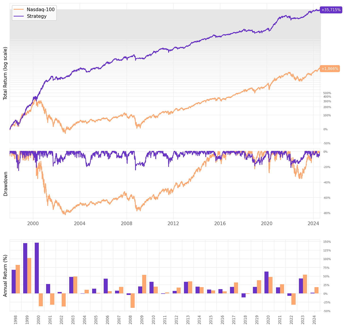
Instead of using 5, let's use 10 as the RSI2 entry threshold. As we have seen earlier, we trade off a bit of edge per a higher number of events (thus increasing the exposure). Here are the results:

Equity and drawdown curves for the strategy using a higher RSI2 entry threshold (10)

Loosening the RSI2 entry threshold worked! The exposure time increased +10 ppts to 93%. As a result:

The annual return increased to 25%, much better than the 18% previous result;
The maximum drawdown got slightly worse, going from 21% to 25%;
The Sharpe ratio improved, reaching 1.23;
As expected, with a loosened entry, we got slightly worse trades, which can be seen with a worse expected return per trade (from +0.88% to +0.79%) and worse payoff ratio (from 0.87 to 0.78);
Nevertheless, we traded more: 239 trades/year on average, vs. 170 obtained earlier.

However, a problem persists: if we look at the annualized return in the past 10 years, the strategy delivered a 16.2% annual return, while the Nasdaq-100 achieved a 17.7% annual return.

How to solve that?

Reducing the number of positions

Naturally, reducing the maximum number of positions should deliver a higher return with higher drawdowns, as we will hold a more concentrated portfolio. Let's see how reducing the maximum number of positions to 4 impacts the results:

Equity and drawdown curves for the maximum number of positions of 4

As expected, reducing the maximum number of positions increased the returns but also the maximum drawdowns:

The annual return now is 34% vs. 25% seen in the previous run;
The maximum drawdown jumped from 25% to 35%;
The Sharpe ratio remained the same at 1.23;

But most importantly, over the past 10 years, the strategy compounded at 24.4% annual return vs. 17.7%.

Thank you for reading Quant Trading Rules. This post is public so feel free to share it.

Looking closer at the recent history

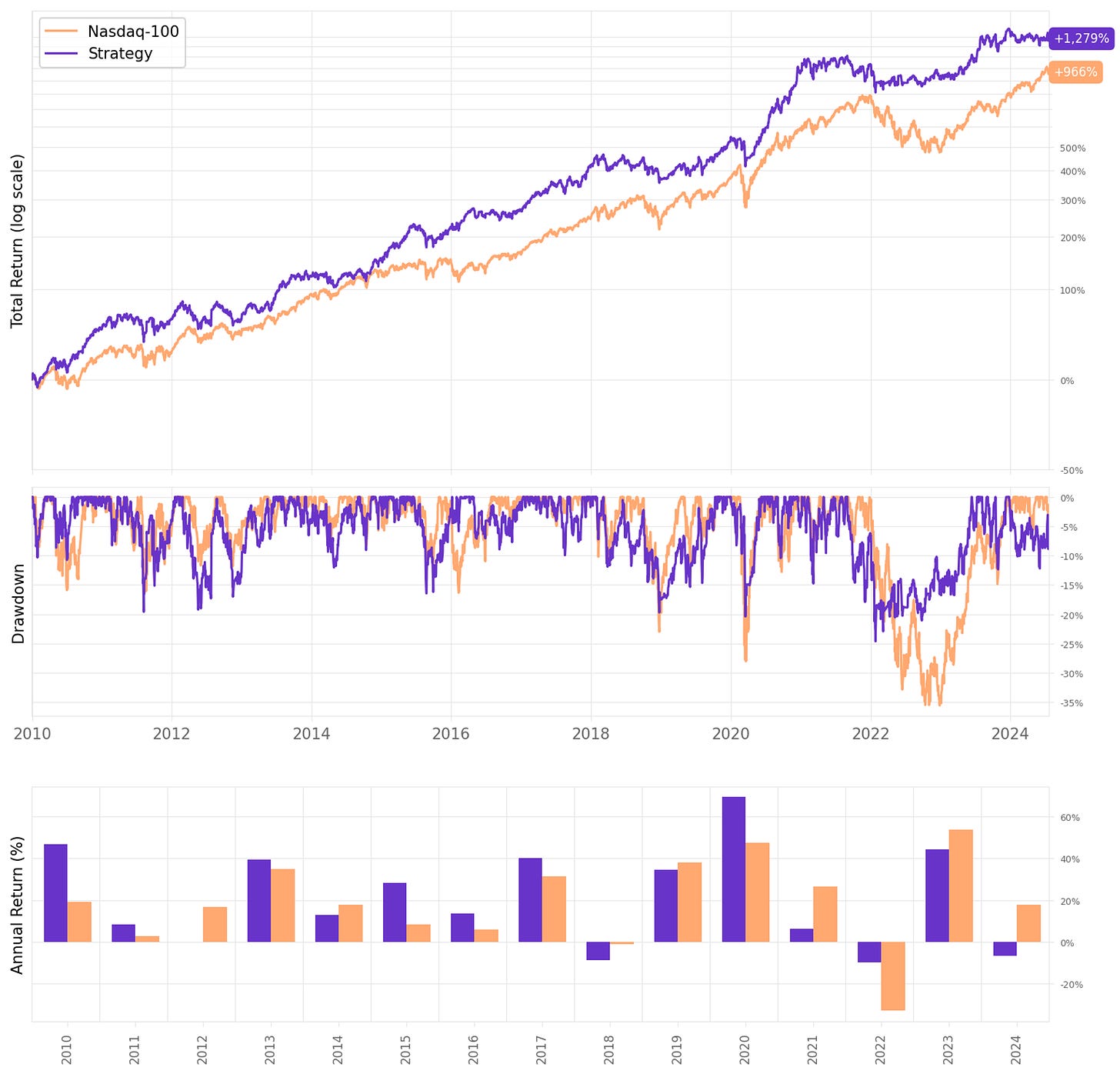
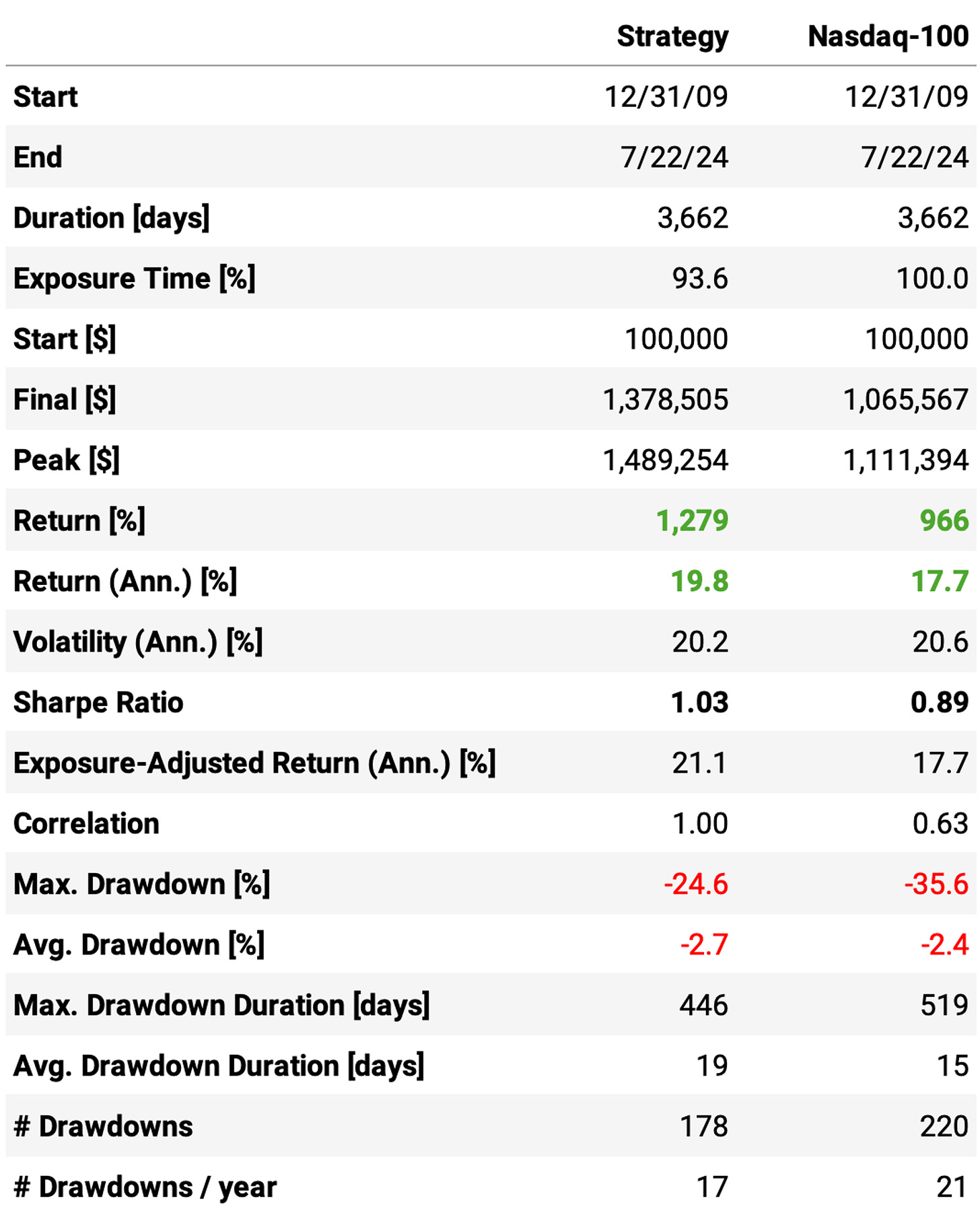
Another terrific input I received from Marsten was to look at returns in recent history when assessing mean reversion strategies like these. They worked great in the 90's and 00's but lost steam after 2010. Let's take a closer look at what has happened since 2010:

Equity and drawdown curves at the recent history.

The strategy is still better than the benchmark, but not that much:

Annualized return is 19.8% vs. 17.7% benchmark;
Sharpe is a bit better at 1.03 vs. 0.89;
The maximum drawdown is better, at 25% vs. 36%.

If we look specifically at the past 4 years, since 2021, the strategy would have lost to the benchmark: The annualized return since 2021 is 7.1% vs. 13.4% of Nasdaq-100.

How do we address this issue?

Trading the mean reversion curve

Seven years ago, Andrew Swanscott shared a great interview with PJ Sutherland in his Better System Trader's podcast. PJ argues that the traditional approach, optimizing a single set of parameters and trading it, is flawed due to parameter instability and luck.

Inspired by Ray Dalio's all-weather portfolio concept, PJ shares his idea of trading the mean reversion curve:

The method involves iterating across a broad spectrum of parameters instead of using a single set;
Then, he constructs an algorithm to automate the diversification across multiple strategies;
According to him, results show more stable performance closely resembling backtested results, reducing the impact of luck.

Let's apply this idea to our system:

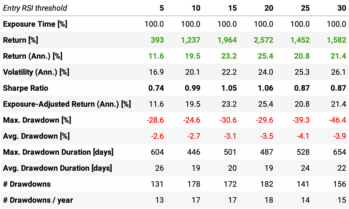
First, let's generate 6 mean reversion portfolios by varying the RSI2 entry threshold: 5, 10, 15, 20, 25 and 30;
Then, let's run a simple optimization algorithm that chooses the weights for these portfolios by maximizing Sharpe.

The 6 different portfolios

Here are the individual performances of the 6 different mean-reversion portfolios. Results are from 2010 on, only the recent history:

Summary of backtest statistics for different levels of RSI2 entry threshold (since 2010)

Now, we can already observe something interesting. When we look at the whole history from 1998 to 2024, we know that the RSI2 entry threshold at 10 is the option with the best edge and the highest expected return. However, when we look at 2010-2024, we see that the entries at 15 and 20 are actually better.

Anyway, this selection includes several sub-optimal portfolios. We will diversify the capital across all of them.

The diversification algorithm

The idea for the diversification algorithm is quite simple:

At the beginning of every period, we will look back N days and find the capital allocation across the 6 portfolios that maximize the Sharpe ratio;
We will keep this allocation fixed for the period;
At the beginning of a new period, we will rebalance, repeating the process.

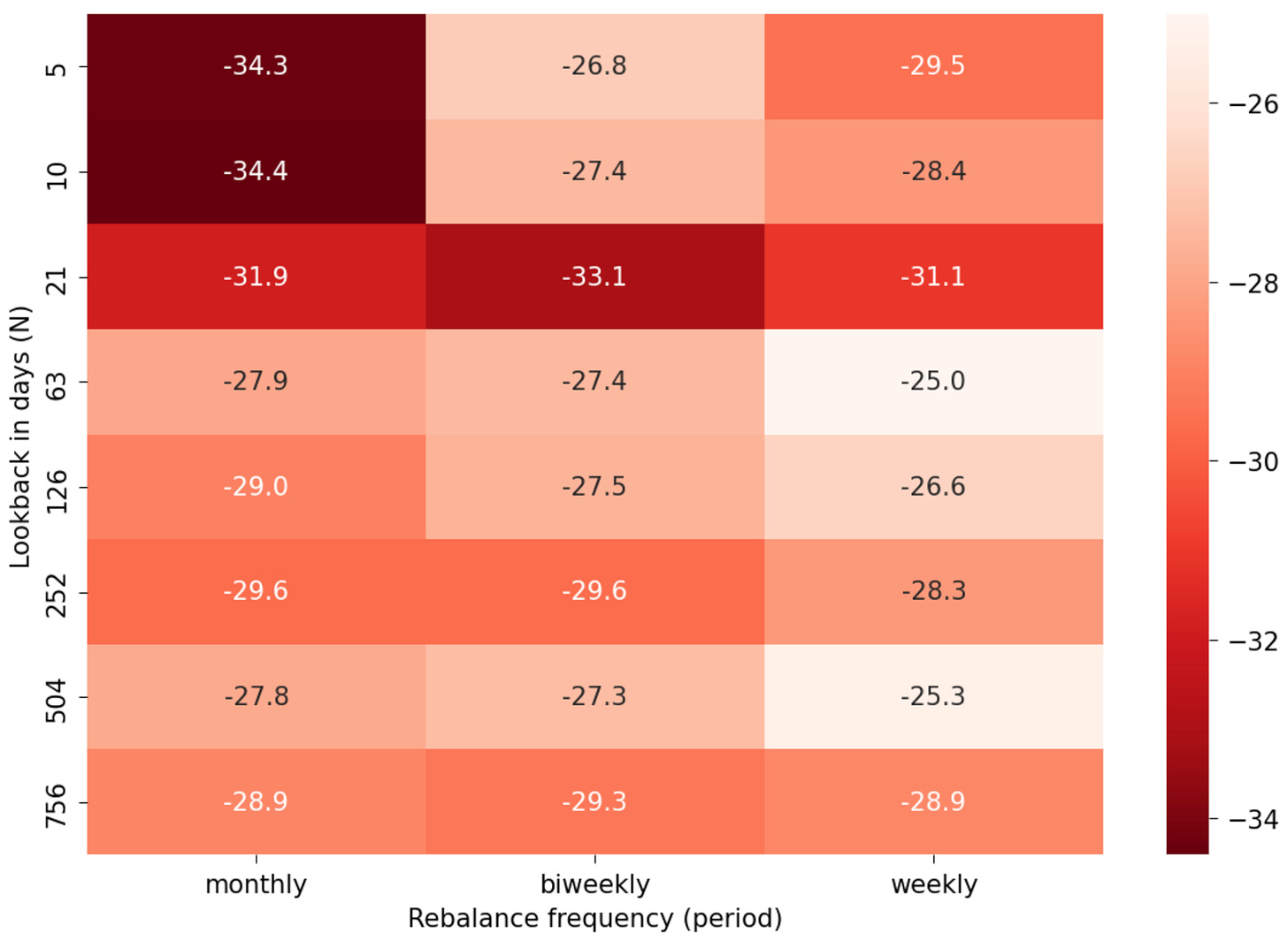
Now, how do we determine the optimal rebalance frequency (period) and look back (N)? Let's try some options:

Periods: monthly, biweekly and weekly;
N: 5, 10, 21, 63, 126, 252, 504 and 756 days.

Here are the results:

Sharpe Ratio for different sets of lookbacks and rebalance frequencies since 2010

Annual returns for different sets of lookbacks and rebalance frequencies since 2010

Maximum drawdowns for different sets of lookbacks and rebalance frequencies since 2010

So, the best combinations are obtained with a lookback period of 5 days, rebalancing weekly. Now, we just choose this combination and we are done, right? Not so fast.

The problem with frequent rebalances

It would be amazing if we could just set the diversification algorithm to look back 5 days and execute the weekly rebalance and expect 35% annual returns. Unfortunately, for this to happen, we would have to close several trades before they trigger the exit rule and open new ones on Monday mornings without friction. That's impossible.

Another way to see it: to execute this frequent rebalances, we would need a perfect continuation between Friday's close and Monday's open. And we know that this is not true. If we look at the distribution of the gap returns between Friday's close and Monday's opens from all stocks in our universe, we see that the mean is 0% as expected, but the standard deviation is 1.4%, with min -89% and max +74%. A lot can happen to stock prices during the weekend.

Thus, although not optimal, we will restrict ourselves to monthly rebalances. In that column, the best look back period is 504 days, or 2 years.

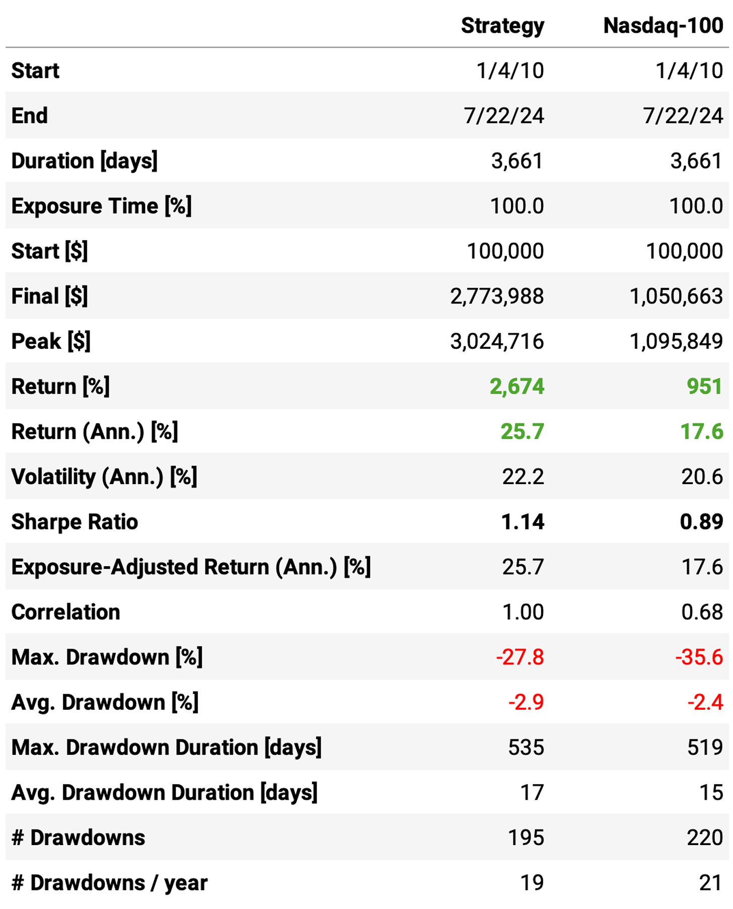
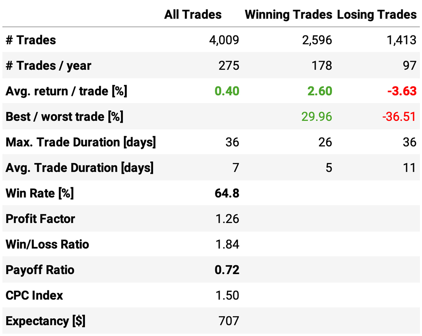
Let's look at this system in detail:

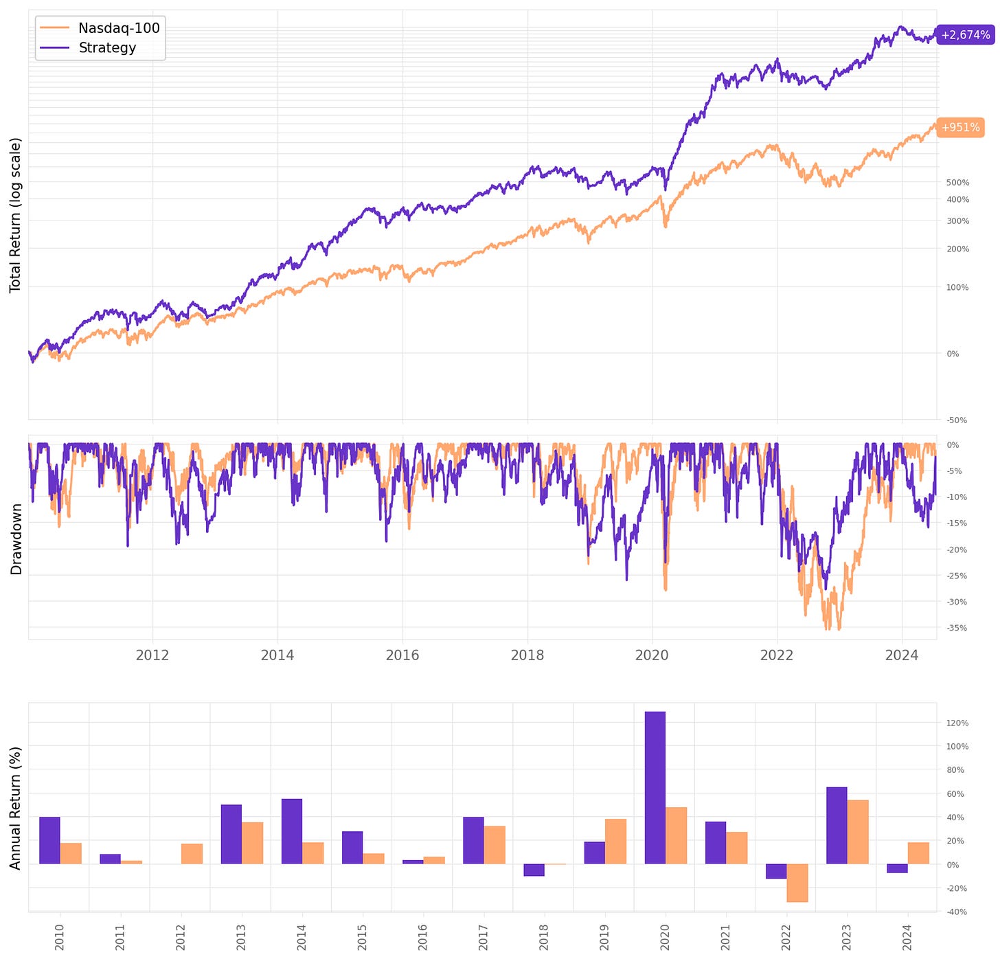
Equity and drawdown curves for the portfolio of mean-reversion strategies, optimized with 504-day look back and monthly rebalance

Highlights:

The strategy achieves 25.7% annual return since 2010, vs. 17.6% benchmark;
Sharpe Ratio is at 1.14, above Nasdaq-100's 0.89 in the period;
Maximum drawdown is also better, at 28% vs. 36%;
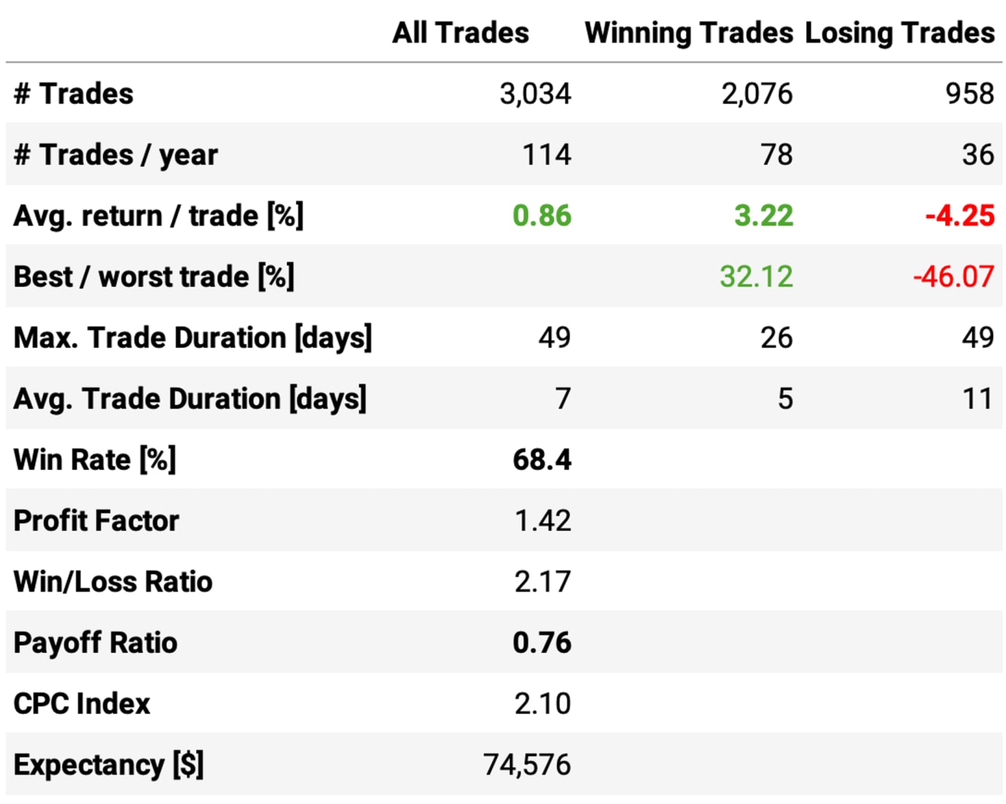
Looking at trade stats, the expected return per trade is +0.40%: the win ratio is 64.8%, with a payoff ratio of 0.72.

If we had traded this strategy since 2010:

We would have had 2 down year (with this year still down so far);
We would have seen 66% of the months positive, with the best at +20.1% (Jul’23);
We would have seen 34% of the months negative, with the worst at -15.2% (May'19);
The longest positive streak would have been 9 months, from Dec'16 to Aug'17;
The longest negative streak would have been 4 months, from Jun'15 to Sep'15.

But what is happening under the hood?

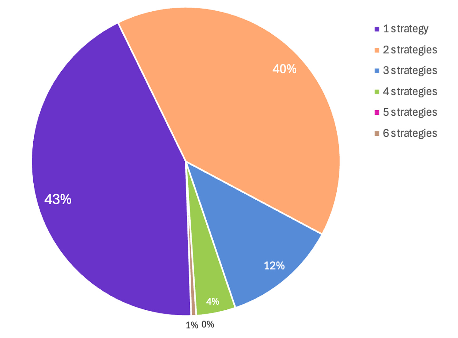
Out of curiosity, let's see to how many strategies the diversification algorithm allocates capital throughout the backtest period:

Distribution of allocation throughout the backtest period

The chart above provides interesting insights:

During 43% of the time, the diversification algorithm is just selecting the strategy with the highest Sharpe amongst the 6 options within the past 2 years, and using it for the next month;
During 40% of the time, the diversification algorithm is allocating the capital to 2 strategies;
The algorithm only allocates to 3 strategies in 12% of the time;
The algorithm almost never allocates capital to 4 or more strategies.

Now, let's look at which are the most used strategies throughout the period:

Strategies’ participation in the portfolio

The data above helps us better understand what is happening:

Although the portfolio spends 43% of the time with a single strategy and 40% of the time with two strategies, these strategies change a lot;
The diversification algorithm makes the strategy with RSI2 entry at 10 the most used strategy, present 49% of the time;
It makes the strategy with RSI2 entry at 25 the least used strategy, present 18%;

The data supports PJ Sutherland's argument: the traditional approach, optimizing a single set of parameters and trading it, is sub-optimal indeed. A much better approach is to iterate across a broad spectrum of parameters instead of using a single set, and automate the diversification across multiple strategies.

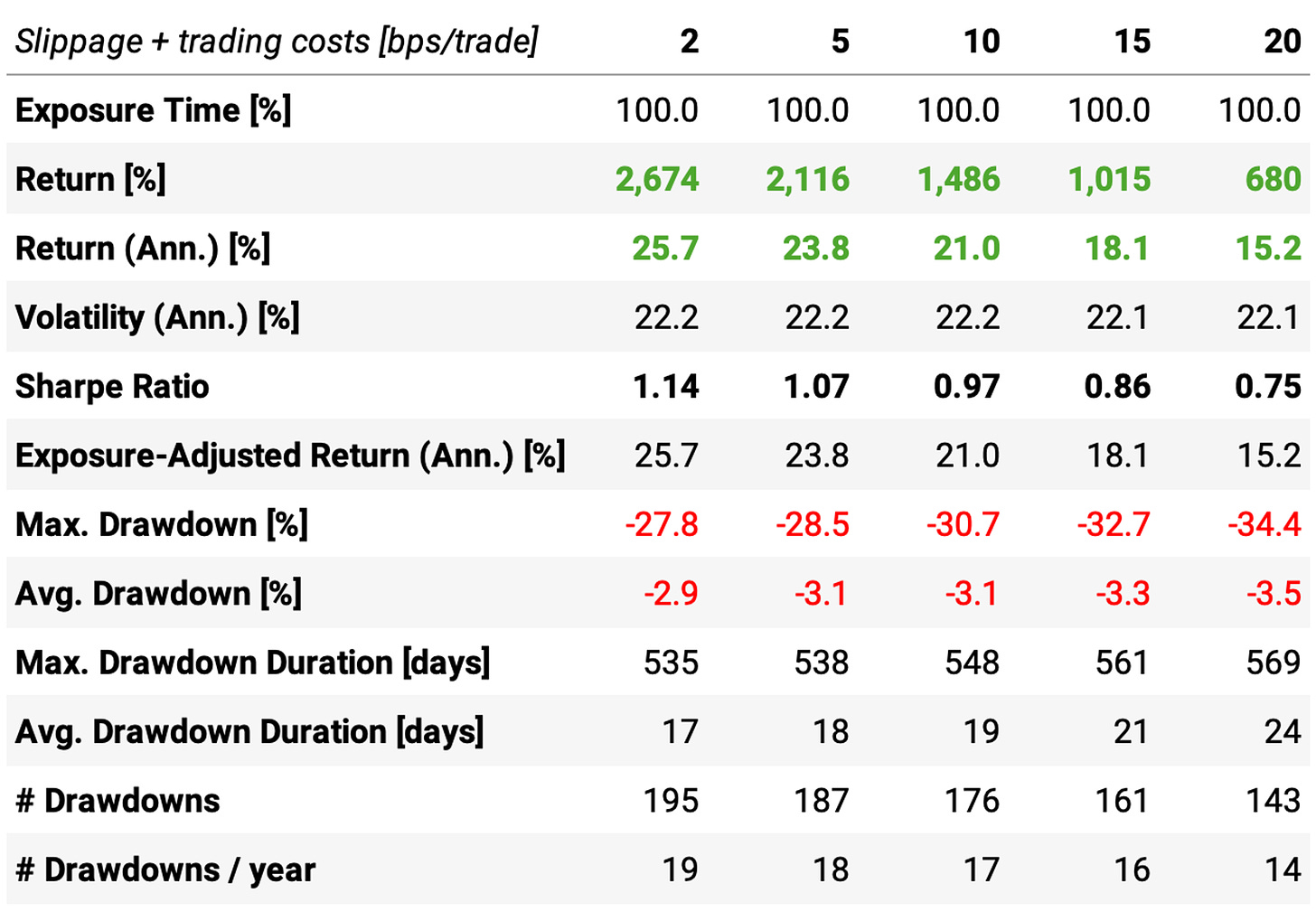
The impact of slippage + trading costs

Finally, we recompute the impact of slippage + trading costs in the key stats:

Final thoughts

Going straight to the point: would I trade this system? Yes. But I am adding changes such that:

Each trade has a higher expected return;
Each strategy better allocates the capital across the daily opportunities;
The system uses a slightly different diversification algorithm;
The system behaves better in market downturns.

I'm not disclosing these additions as they take this strategy to production level. But I'm sure some will figure them out. :)

I want to end this article by thanking Marsten Parker, Andrew Swanscott, and PJ Sutherland. This article was only possible because these great systematic traders shared their thoughts and ideas.

As usual, I'd love to hear your thoughts about this approach. If you have any questions or comments, just reach out via Twitter or email.

Also, if you want to implement this strategy (or any other strategy) and need help, just let me know.

Cheers!