Trading ETFs while fear and greed rise
A system to scaling into positions that deliver 21% annual returns since 1999
The idea
"The first principle is that you must not fool yourself, and you are the easiest person to fool.” Richard Feynman
Richard Feynman was one of the great scientists and physicists of our time, truly one of the great minds of humanity. This is one of my favorite quotes from him. It emphasizes the importance of intellectual honesty and self-awareness in scientific inquiry and in life in general.
We have a tendency to deceive ourselves, either consciously or unconsciously. He cautions against cognitive biases, wishful thinking, and self-delusion, which can cloud our judgment and lead to erroneous conclusions.
Feynman stresses the need for humility and critical self-reflection. Scientists and individuals alike must constantly question their assumptions, challenge their beliefs, and be open to revising their views in the face of new evidence. This quote underscores the importance of skepticism, rigorous self-examination, and a commitment to seeking truth without succumbing to personal biases or preconceptions.
His Caltech’s 1974 commencement address is a masterpiece.
Listening to Andreas Clenow on
, hosted by and (amazing interview, strongly recommend to all - here's the link) made me think of him. Especially when he shared ideas like these:“You don't trade somebody else's model without understanding what it is and what it does. You need to be cynical enough not to trust any sort of backtesting software—whatever comes out of it—and do your own math.”
As you might have already noticed, I strongly believe in that.
In another insightful part of the interview, Andreas emphasized that both trend-following and momentum strategies are valuable building blocks rather than complete solutions. They should be part of a diversified portfolio rather than standalone strategies.
He highlights the importance of creating a well-rounded portfolio using various strategies as building blocks to achieve overall investment goals rather than relying on a single strategy.
I was already a fan (of both Andreas and the podcast) and became even more impressed. I strongly recommend Andreas’ books and listening to
Podcast.This week, we will test the idea based on the TPS strategy from Larry Connors's book Buy the Fear, Sell the Greed.
T: Time
P: Price
S: Scale-In
TPS identifies when an ETF is oversold and averages into the position as it becomes more oversold.
Here are the TPS rules on the long side:
The ETF is above its 200-day simple moving average.
The 2-period RSI is below 25 for two days in a row. Buy 10% of your position.
If prices are lower on the close than your previous entry price, any day you’re in the position, buy 20% more of your position (you’re averaging in).*
If prices are lower on the close than your previous entry price, any day you’re in the position, buy 30% more of your position.*
If prices are lower on the close than your previous entry price, any day you’re in the position, buy 40% more of your position.*
Using this 10%, 20%, 30%, 40% scaling-in approach (also known as 1-2-3-4), you now have a full position in a very oversold ETF.
*Do not take a new position anytime the ETF closes under the 200-day MA.
Exit when the 2-period RSI closes above 70.
As highlighted by Cleanow, we should not rely on a single strategy. So, consider this strategy as a building block to be used in a portfolio of strategies. And most importantly, do your own math.
Data considerations
This article uses Norgate data. It's a great survivorship-bias-free dataset that contains thousands of active and delisted ETFs since the 1990s.
In the book, Connor recommends focusing on unleveraged, non-inverse ETFs. This is simple to filter with Norgate dynamic watchlists. However, even after filtering, the list might include ETFs that contain derivatives (in other words, highly leveraged). Also, the book is not clear whether we should include ETNs or not.
I'm using ETFs only, not including ETNs. Also, I developed a small script that checks every ETF (search online) to determine if it contains derivatives, excluding the ones that do.
The edge
Let's start by verifying the edge in buying all events when an ETF's (unleveraged, non-inverse) 2-period RSI crosses below 25 for two consecutive days and selling when it crosses above 70, provided its closing price is above its 200-day SMA. These returns consider the 1-2-3-4 scaling approach.
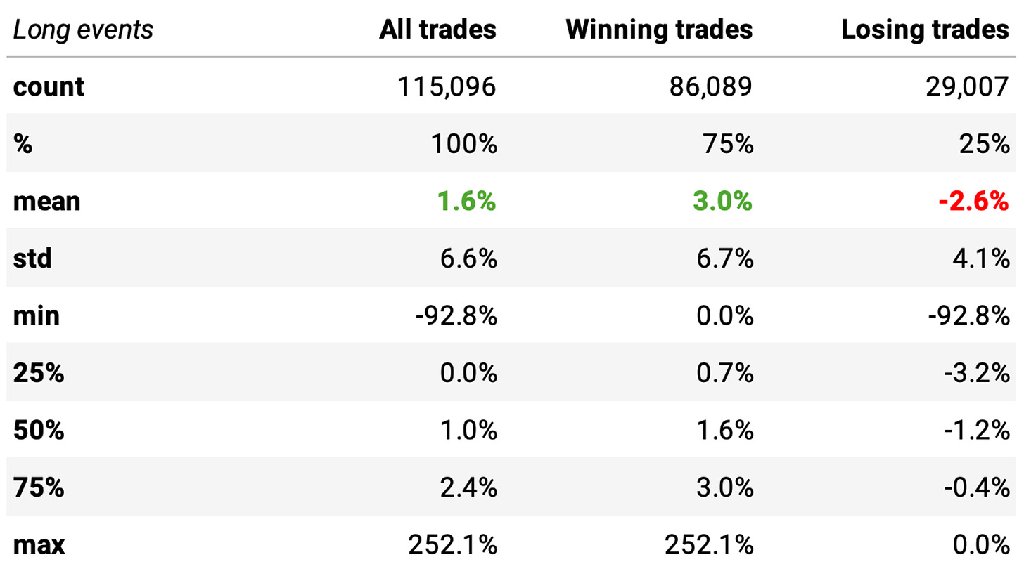
There's a good 75% probability of success, although the numbers are inferior to what was presented in the book.
Also, the payoff ratio is positive: winning trades are expected to return +3.0% while losing trades -2.6%. Overall, the expected return per trade is +1.6%.
Now, let's check the stats of non-events. We define non-events as buying ETFs whenever their 2-day RSI closes above 25 in either of two consecutive days and holding the trade for 8 days (which is the median duration of the trades obtained in the events).
Curiously, although we see a coin flip (51% probability of success), we observe a small positive expected return of +0.5%. That's probably because of the positive drift observed in financial markets. Anyway, the P-value is well below 0.05: the means of the two distributions are significantly different. So, we have an edge.
Occurrence of events
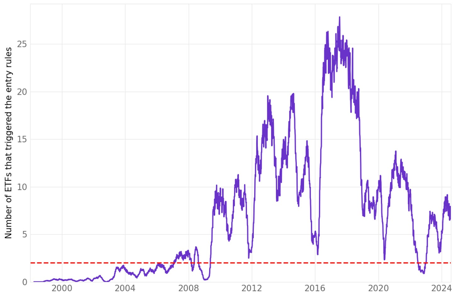
Before we start the experiments, let's check how many ETFs have triggered the entry rules since 1998. To remove small illiquid ETFs, we will only look at ETFs with a turnover higher than USD 100 million/day on average.
As the chart shows, plenty of ETFs triggered the entry rules, especially after the 2008 crisis.
The strategy
The strategy was well described at the beginning of the article. We will focus only on the long side. Additional important details:
We will only trade ETFs with a turnover higher than USD 100 million/day on average;
We will start with maximum positions = 1, which means we will only trade if we are not already carrying a position; if we are, we will ignore any opportunities;
We will trade always at the next opening;
We will start with denominator 10 in the 1-2-3-4 scaling system. This means no leverage:
First position will take 1 / 10 of the capital allocated to that trade (10%, sum 10%);
Second position, if needed, will take 2 / 10 (20%, sum 30%);
Third position, if needed, will take 3 / 10 (30%, sum 60%);
Fourth position, if needed, will take 4 / 10 (40%, sum 100%).
Later, to apply leverage, we will just reduce the denominator accordingly.
Experiments
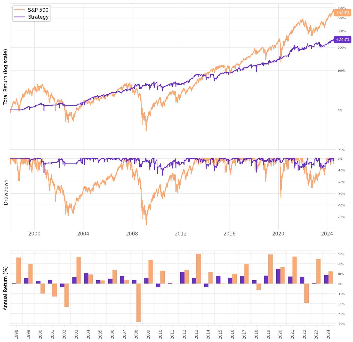
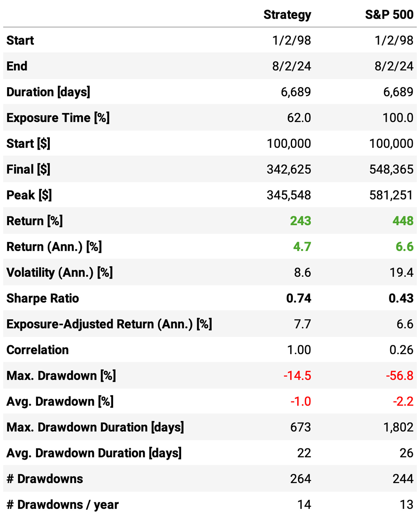
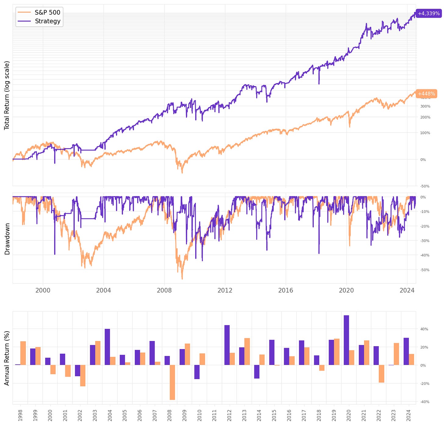
As mentioned, we start with maximum positions = 1 and denominator = 10 in the 1-2-3-4 scaling system (i.e. no leverage):
Highlights:
The annual return is 4.7% vs. 6.6% the benchmark in the period;
The exposure is only 62%; exposure-adjusted annual return is at 7.7%;
Sharpe ratio is 0.74, much better than the 0.43 of the S&P 500;
Maximum drawdown is at 14.5%, well below the 57% of the benchmark;
The expected return/trade is +1.0%, with an win rate of 76%;
Profit factor is at 1.82; win/loss ratio is over 3; however, payoff ratio is 0.73.
Although the exposure time is 62%, the capital was not well employed:
Because of the 1-2-3-4 system, on an average day, the expected % of cash sitting idle in the account was 90%;
In only 16% of the days, 50% or more of the capital was allocated.
How can we improve the capital allocation?
Improving the capital allocation
Let's look closer at how the capital is being employed:
The chart above is telling:
In 38% of the days, 100% of the cash was sitting idle in the account;
In 68% of the days, we had the first leg of the position executed;
In 31% of the days, we had the second leg of the position executed;
In 17% of the days, we had the third leg of the position executed;
in 9% of the days only, we had all the legs of the position executed.
This means that 83% of the time, we either had no trades or had a trade in stages 1 or 2 of the 1-2-3-4 system.
So, based on the data above, we will start improving the capital allocation by changing the denominator parameter in the 1-2-3-4 system to 3. This means that, for every trade:
First position will take 1 / 3 of the capital allocated to that trade (33%, sum 33%);
Second position, if needed, will take 2 / 3 (67%, sum 100%);
Third position, if needed, will take 3 / 3 (100%, sum 200%);
Fourth position, if needed, will take 4 / 3 (133%, sum 333%).
With this system, 83% of the time, we expect either no trades or 100% of the capital employed. 17% of the time, in stages 3 and 4 of the 1-2-3-4 system, we will use leverage.
Here are the results:
Adding leverage worked:
The annual return increased to 15.4%, more than twice the benchmark;
The Sharpe ratio also increased, now at 0.78;
However, as expected, the maximum drawdown also increased, reaching 44%;
The exposure time is exactly the same as the trade stats.
The better numbers result from improved capital utilization: now, on average, on a given day, 67% of capital sits idle in the account vs. the previous 90% value.
But we can do better. We can improve these drawdowns.
Diversification
Up to now, we have been using the maximum number of positions equal to 1. Now, let's improve this number to 5. So, at the beginning of every trading session:
We will split the total value into 5 portions: these will be the total capital available to every single trade;
For every single trade, we will apply the 1-2-3-4 system as described previously, keeping the denominator factor as 3 (i.e., using leverage) and scaling the positions accordingly;
We will carry a maximum of 5 positions at any given time: if we are carrying less than 5, we will look for opportunities (ETFs with entry signal triggered), sort them by turnover (descending), and fill in the trades until all the 5 slots are filled;
As the exit signal is triggered in every trade, we will close the positions and re-open the slots to be filled again.
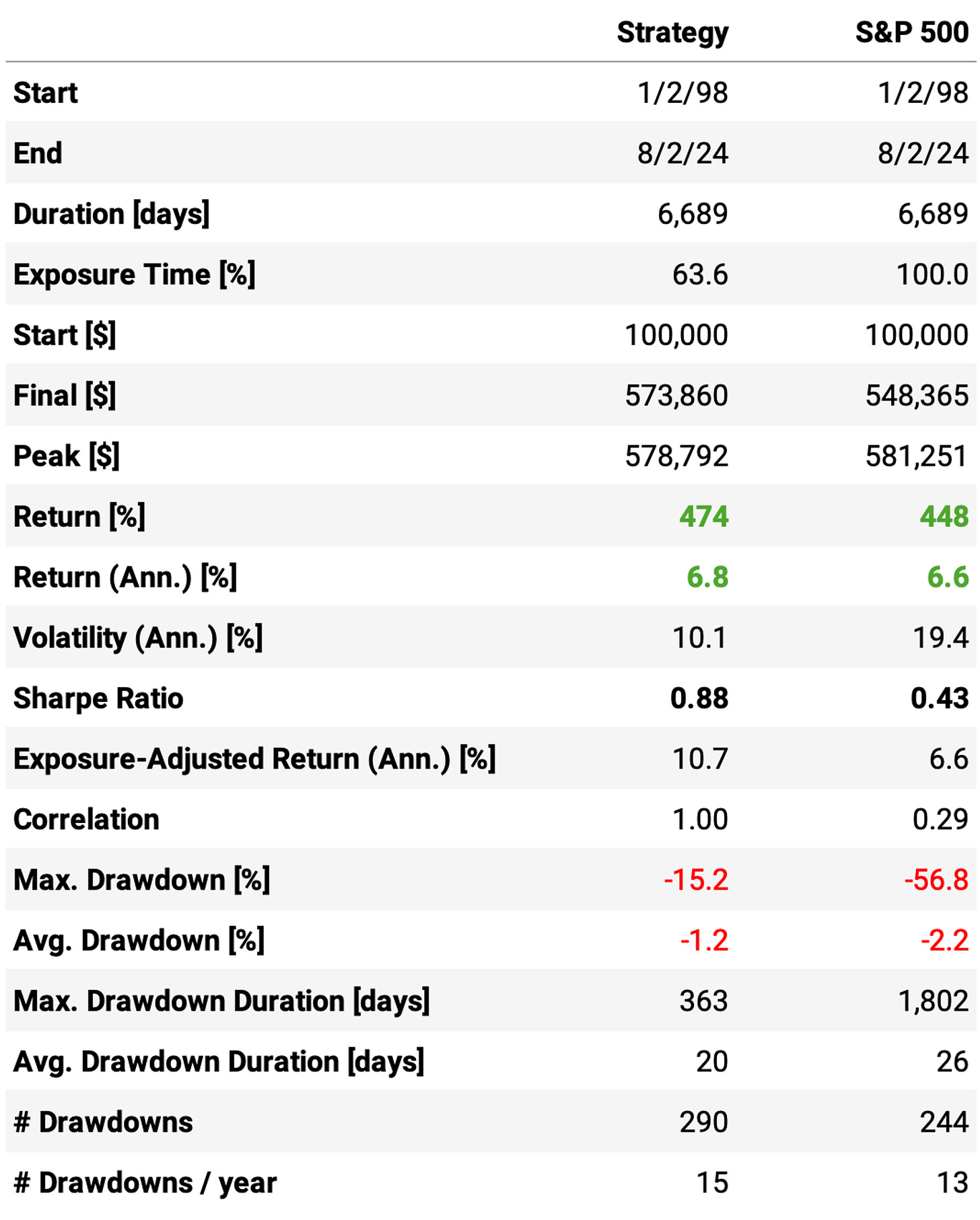
Applying diversification leads to this:
Highlights:
Increasing the maximum number of positions to 5 led to an annual return of 6.8%, about the same as the S&P 500;
However, we achieved much better risk-adjusted returns: Sharpe ratio reached 0.88, twice as much as the benchmark;
The maximum drawdown also decreased, now at 15% vs. 57% the benchmark;
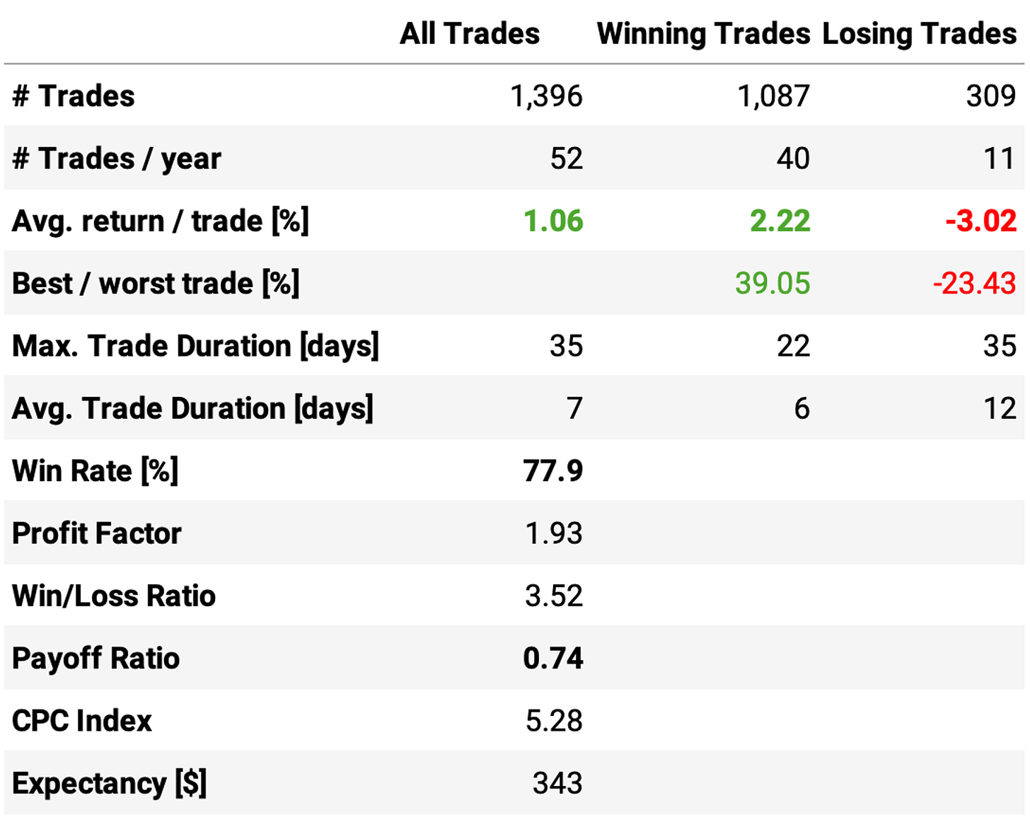
The trade stats improved a bit: now the win ratio is at 78%, the profit factor of 1.93, and the win/loss ratio at 3.52;
Now, the system is trading on average 52 times/year, or once a week.
However, capital utilization got worse: now, on an average day, 80% of the capital sits idle in the account. That's because it's not every day we can find 5 ETFs triggering the entry rules. How can we fix that?
Adjusting the denominator factor
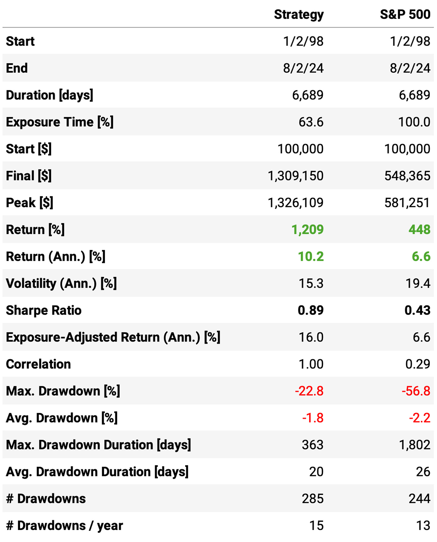
We already know how to improve capital utilization: we just need to reduce the denominator factor. Let's use 2 instead of 3:
Again, we achieved the desired result:
The annual return increased to 10.2% vs. 6.8% in the previous run;
Sharpe ratio remained twice as big as the S&P 500's at 0.89;
The maximum drawdown increased to 23%, which is acceptable and way better than the benchmark's (57%).
Nevertheless, a 10.2% annual return is below the minimum we strive to reach (15%). Further increasing leverage (using denominator factor 1 instead of 2) would not be ideal, as it would result in a few days with extremely high leverage. How can we improve further?
Long & short portfolio
Our last trick is to add a short leg. The short side will work exactly the same as the long side but in reverse. Here are the rules for the TPS short:
ETF is below its 200-day simple moving average;
The 2-period RSI is above 75 for two days in a row. Sell short 10% of your position;
If prices are higher on the close than your previous entry price, any day you’re in the position, sell short 20% more of your position (you’re averaging in)*;
If prices are higher on the close than your previous entry price, any day you’re in the position, sell short 30% more of your position*;
If prices are higher on the close than your previous entry price, any day you’re in the position, sell short 40% more of your position*;
*Do not take a new position anytime the ETF closes above the 200-day MA.
Exit when the 2-period RSI closes below 30;
We will trade both the long and short portfolios in parallel. We will use a maximum of 3 positions for the long portfolio but 6 positions for the short portfolio. That's because we want more diversification in the short side to protect us from outliers.
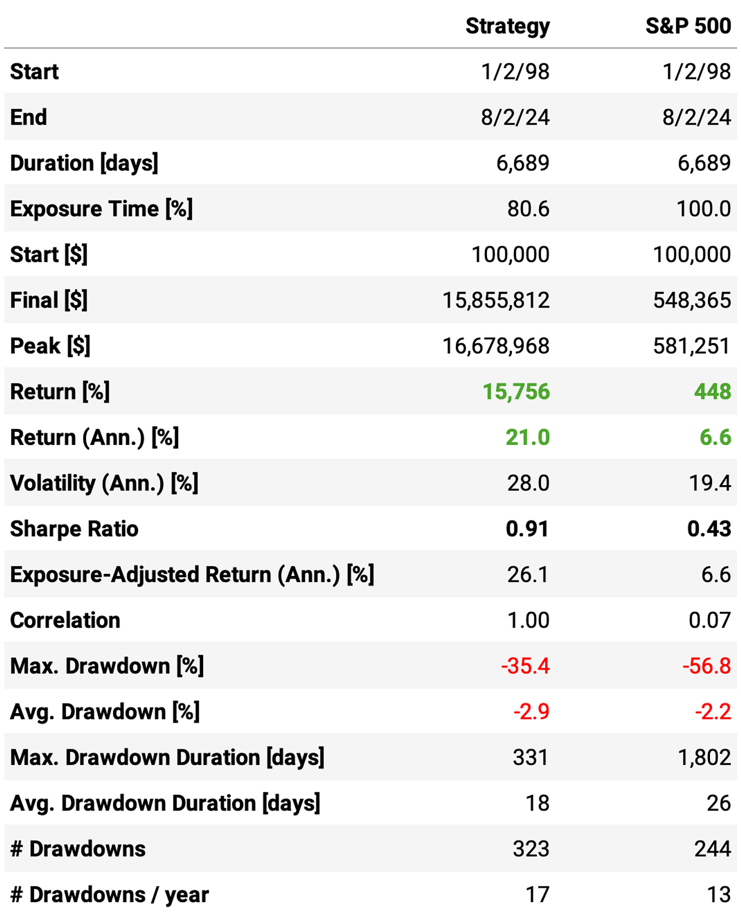
Here are the results:
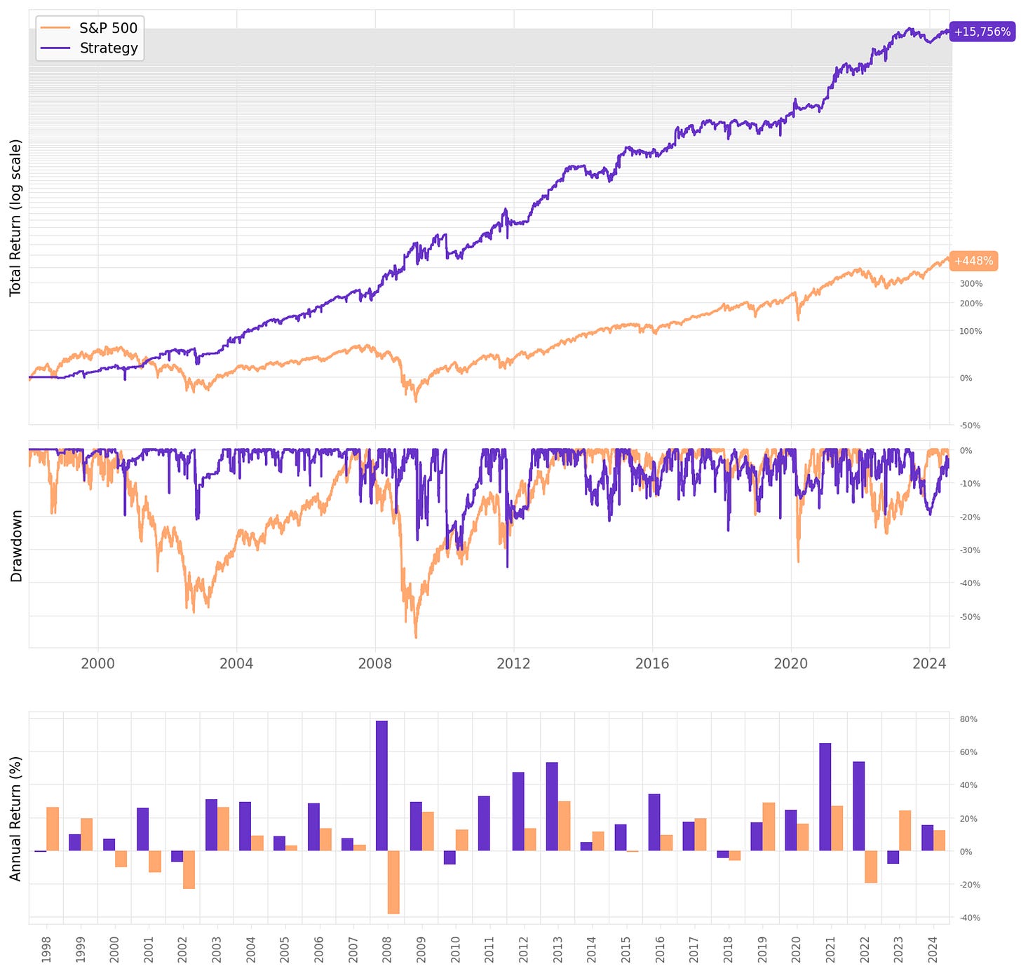
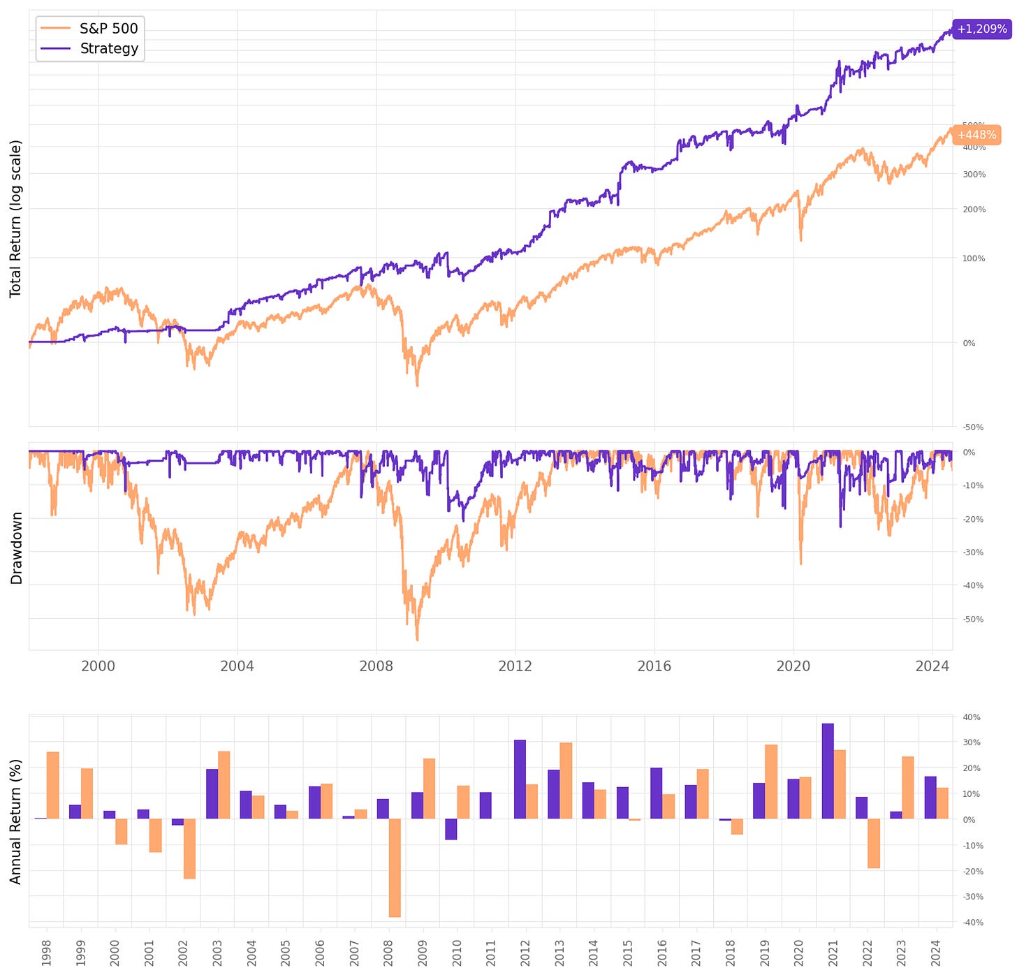
The implemented changes, adding the short leg and changing the max positions, worked as intended:
Annual returns achieved 21.0%, over 3x the benchmark;
Sharpe ratio of 0.91, over 2x the benchmark and the best value in all our experiments;
Maximum drawdown reached 35%, which is above what we want (20%) but much better than the 57% of the benchmark;
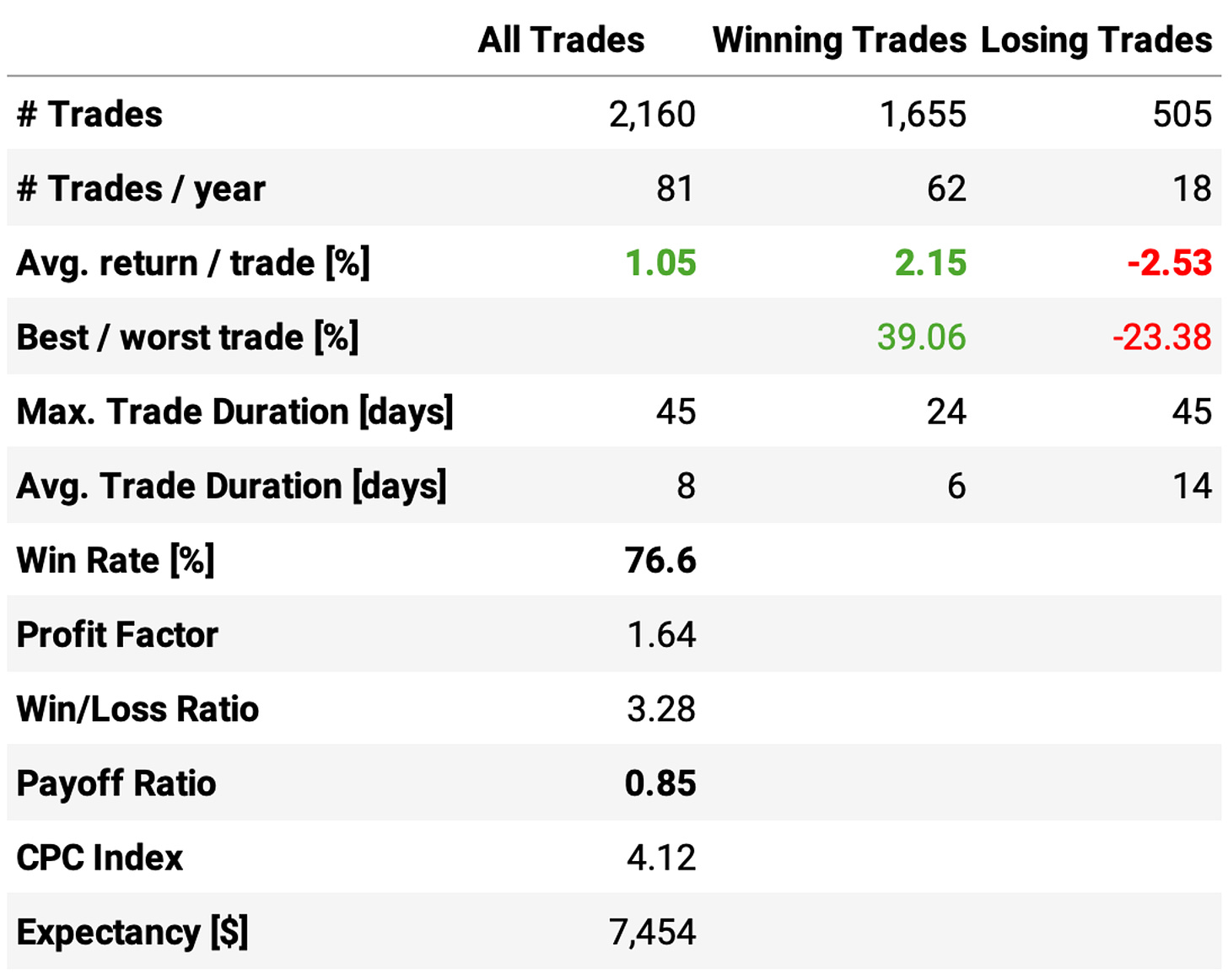
Trade stats continued strong, with 81 trades/year (about 3 trades every 2 weeks) @ 77% win rate, with an expected return/trade of +1.05% and a payoff ratio of 0.85.
If you want lower drawdowns, they can be easily achieved by using 4-8 max positions instead of 3-6. Finally, let's look at what would have happened month by month since 1999:
If we had traded this strategy since 1999:
We would have had 4 down years in 26;
We would have seen 68% of the months positive, with the best at +30.9% (Sep’16);
We would have seen 32% of the months negative, with the worst at -29.1% (Jan'10);
The longest positive streak would have been 17 months, from Apr'12 to Aug'13;
The longest negative streak would have been 4 months, from Aug'21 to Nov'21.
Final thoughts
I like this strategy. The maximum drawdown is still a bit higher than what I like, but I think the general idea of the TPS, with the tweaks and changes added here, is a good start to further improvements.
Before trading it, here are some improvement suggestions:
Try a different way to select ETFs to trade. So far, I've just filtered unleveraged and non-inverse ETFs and applied a liquidity filter. We can think of more interesting ways of creating lists (e.g., at the beginning of every year, dynamically create a list of the top 500 ETFs that are not highly correlated to each other);
Try different universes rather than ETFs (stocks belonging to indices such as Nasdaq-100, S&P 500, Russell 3000, etc.);
Try different exits.
As usual, I've considered 2 basis points in slippage + trading costs in all trades. We should obviously expect a lower return for higher costs. I also did not include any costs related to leverage or gains related to capital sitting idle in the account. Adding those would increase the complexity of the tests and add a bunch more assumptions, and I suspect one would offset the other. And the objective is to give you the overall idea of the strategy.
This idea, as with any other, should be seen as a building block upon which we should build a portfolio of strategies. No single strategy will work 100% of the time in all market regimes. Now, a portfolio of uncorrelated strategies might do the trick ;)
Again, I would like to thank
for their amazing podcast and Andreas Cleanow and Larry Connors for openly sharing their ideas. This article was only possible because these great systematic traders generously shared their knowledge and insights.As usual, I'd love to hear your thoughts about this approach. If you have any questions or comments, just reach out via Twitter or email.
Also, if you want to implement this strategy (or any other strategy) and need help, just let me know.
Cheers!







Fascinating. I tested this mean reversion with scaling approach, and it works well across equities and fixed income sector futures. Especially in US markets. The rules don't work in commodities sectors. It'd be nice to see how it works in stocks mean reversion strategies like your Nasdaq 100 strategy.
Interesting ideas. Thanks for publishing and keep up the great work. Have you tried reducing the universe of ETFs to a logical set? For instance does it work on just the SPY sector ETFs or the iShares global ETFs?