Statistical Arbitrage

Can we get over 20% of annual returns uncorrelated with market risk?

Ray Dalio, founder of Bridgewater Associates, the largest hedge fund in the world

The idea

"The holy grail of investing is to have 15 or more good, uncorrelated return streams.” Ray Dalio.

I find Ray Dalio's story truly inspiring. From founding Bridgewater Associates in his two-bedroom apartment and growing it into the largest hedge fund in the world to publicly sharing the principles that guided him—what he did right and wrong throughout the years—Dalio has always prioritized transparency and self-reflection. His journey is marked not just by his success but by his willingness to openly acknowledge his mistakes, learn from them, and turn those lessons into tools for others.

The greatest obstacle to rational decision-making, he found, was “the ego barrier,” the desire to prove oneself right and others wrong, even in the face of evidence to the contrary. I believe so many people on Twitter would profit from applying his principles. Anyway…

As he openly shares his thoughts, there are many great quotes from him. One of the greatest is about the holy grail of investing, according to him: having 15 or more good, uncorrelated return streams.

So far, all ideas I have shared are somewhat positively correlated with the market. This week, I am sharing the overall gist of a statistical arbitrage model I've been working on for the past weeks.

A key characteristic of statistical arbitrage is the market neutrality. Stat arb strategies typically aim to be market-neutral by balancing long and short positions, reducing exposure to overall market movements, and focusing on the spread between assets. This will be one of the key focus of this idea.

Here's our plan:

1. First, we will introduce statistical arbitrage, explain some of its most popular variations, and select one on which to build our model.

2. Second, we will explain our model and the approach used to create it.

3. Then, we will prove our model has a statistical edge.

4. Next, we will devise a strategy that profitably uses our model.

5. Finally, we will perform some backtest experiments and analyze the results.

This is a model I've been developing for production. So, as usual, I will share the overall gist but not every single detail. You can fill in the blanks using your creativity.

Statistical Arbitrage

My goal is not to provide a full review of statistical arbitrage. However, defining the term is a good introduction to our strategy.

Statistical arbitrage can be defined as a quantitative trading strategy that identifies short-term pricing discrepancies between financial instruments based on statistical models, which aim to detect and capitalize on temporary deviations from expected price relationships or historical norms. The strategy often balances long and short positions to remain market-neutral and aims for mean reversion or relative convergence to generate returns.

Key Characteristics of Statistical Arbitrage

• Market Neutrality: Stat arb strategies typically aim to be market-neutral by balancing long and short positions, reducing exposure to overall market movements, and focusing on the spread between assets.

• Mean Reversion: The strategy often assumes that price deviations between pairs or groups of assets are temporary and will revert to a mean or historical relationship.

• Relative Value Focus: Rather than forecasting absolute price movements, statistical arbitrage relies on relative mispricing. It profits from the convergence of misaligned prices between correlated or cointegrated assets.

• High Volume and Short Holding Periods: Stat arb strategies often involve a large number of trades over short holding periods, attempting to capture small, frequent gains.

• Data-Driven Models: These strategies use advanced statistical techniques, such as machine learning, regression analysis, and time series models, to identify profitable opportunities based on historical data patterns.

• Risk Management: Statistical arbitrage incorporates risk management techniques to limit losses from unpredictable deviations. Strategies are tested and backtested rigorously to ensure robustness.

Example Applications

• Pairs Trading: A classic stat arb strategy that identifies two historically correlated assets (like stocks in the same sector) and trades on temporary deviations in their price relationship;

• Multi-Asset Portfolios: Long and short positions are taken across a basket of stocks based on factor models;

• Machine Learning-Based Predictions: Using models to predict short-term returns and rank assets, then taking offsetting long and short positions based on relative rankings.

The model

Our strategy is based on machine learning-based predictions. We will develop a simple model to predict short-term returns and rank assets. Then, we will long the top predictions and short the bottom ones, continuously creating market-neutral portfolios.

The dataset and features

I use Norgate data, a great survivorship-bias-free dataset. To collect data points, I settled on the Russell 3000 universe (current and past).

For features, I use:

• Rates of change for different windows (short, mid, and long terms, up to a year);

• Distances from the last price to moving averages of different lookback windows (also up to a year);

• How far the last volume is from the past 6 months average

All distances are computed in percentages so we can compare apples to apples. Then, they are properly standardized.

For target, we get the next 3-days return.

Before training and using the model, we transform the returns in the features and the target into log returns.

Algorithm options

I formulated this problem as a regression problem. The trained model will try to predict the magnitude of the log return for the next 3 days.

Several possible algorithms exist: simple linear regression, Ridge regression, Lasso regression, Elastic-Net, and more advanced models like Decision Trees, Random Forests, and Gradient Boosting Machines (GBM). We could also leverage ensemble techniques, such as XGBoost or LightGBM, known for their strong performance on regression tasks with structured data. Each model has its strengths; for instance, linear regression provides interpretability, while regularization methods like Ridge and Lasso help prevent overfitting by penalizing large coefficients. Meanwhile, tree-based models can capture non-linear relationships within the data, which may improve predictive accuracy in financial time series data.

The training process

To train the model, we will use the sliding window technique, with 10 years of lookback, retraining the model at the beginning of every year:

• 2024 model: trained with data from 2014 to 2023;

• 2023 model: trained with data from 2013 to 2022;

• 2022 model: trained with data from 2012 to 2021;

• So on and so forth.

The edge

After training the model, the first question we want to answer is: what is the edge of using such a model?

To analyze that, we:

• Compute the prediction for every stock in the universe for every day since 2010;

• Compute the realized future returns for every stock;

• Assign a decile to each stock every day;

• Aggregate by decile and annualize returns.

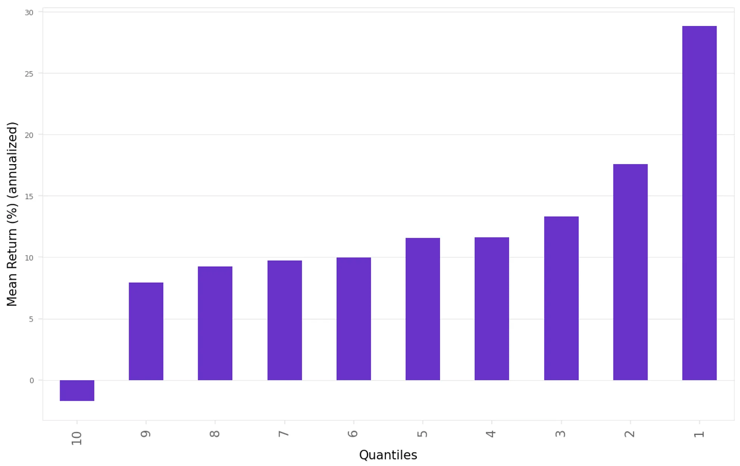
Here's what we found:

Mean return across deciles

This is precisely what we expected:

• The top-decile stocks (1st decile) show the highest returns

• The bottom-decile stocks (10th decile) show the lowest (negative) returns

• This is what we need to create a long-short portfolio

The strategy

Here are the rules to use our model. We will split our capital into three equal portfolios. Each portfolio will be rebalanced every 3 days. The only difference between each of them will be the starting date. For each portfolio:

• At the opening of a 3-day cycle, we will use the model to compute the next 3-day log returns for all Russell 3000 constituents on that date;

• We will go long on the top 20 predictions and short on the bottom 20 predictions;

• We will cap any position in no more than 3% of the available capital;

• We will exclude penny stocks (price below $1), biotech stocks, and meme stocks;

• After 3 days, at the opening, we will close all the positions and repeat the process.

That's it. It is crucial to exclude penny stocks, biotech stocks, and meme stocks, as these stocks show the largest overnight price swings. A short position in them might severely impact the returns. Identifying penny stocks and biotech stocks is trivial (Norgate has a great classification system). Identifying meme stocks programmatically is not that complicated: a good method can be found here.

Throughout all the experiments, we will consider 10 basis points in trading costs in every trade.

Experiments

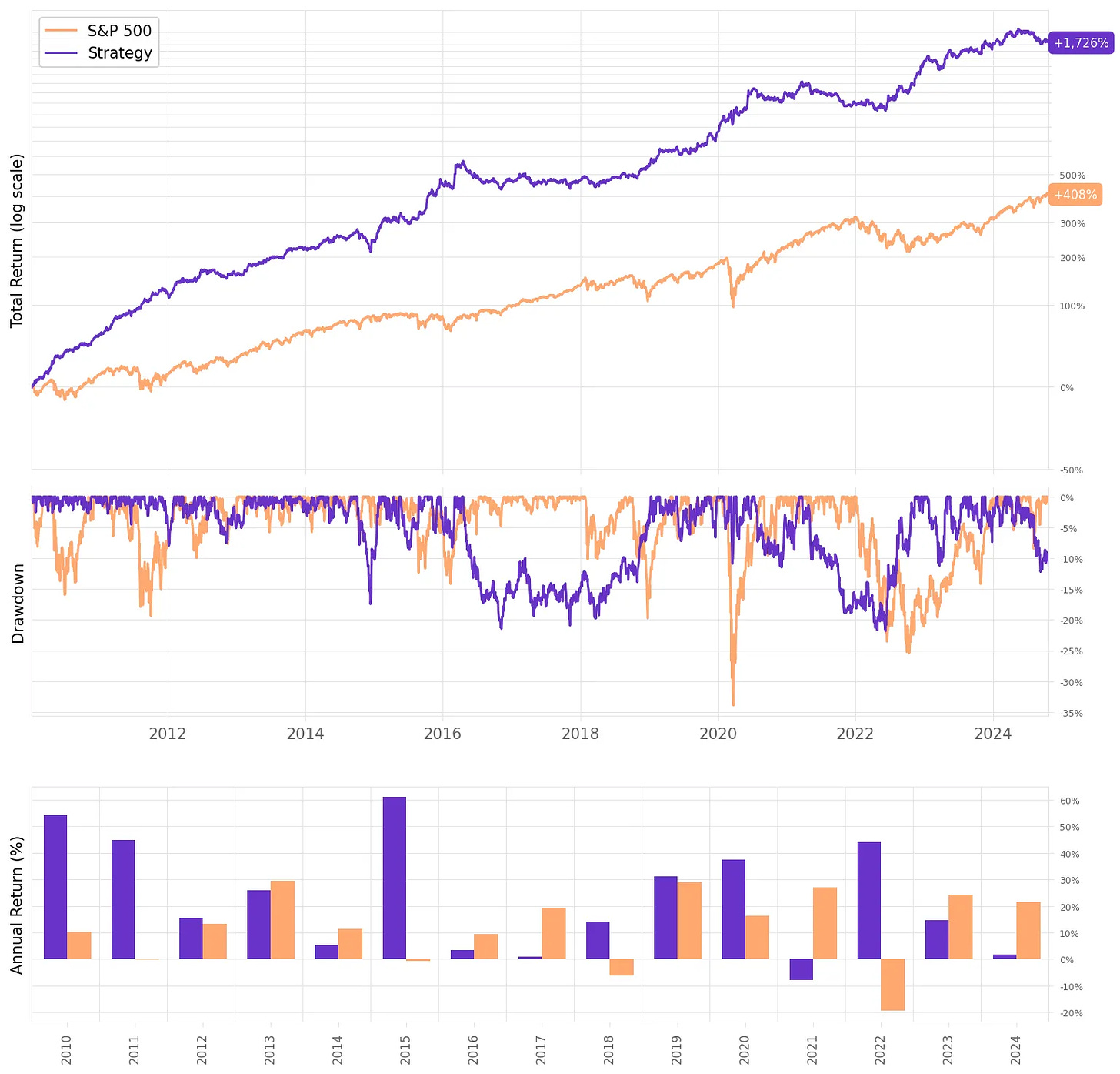
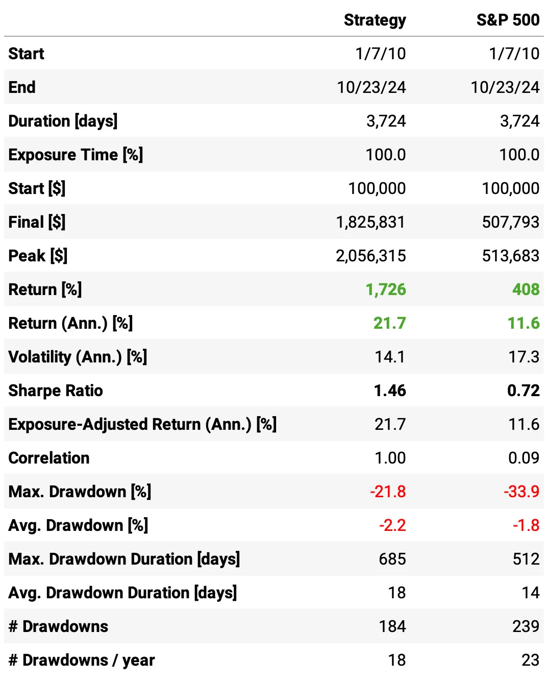
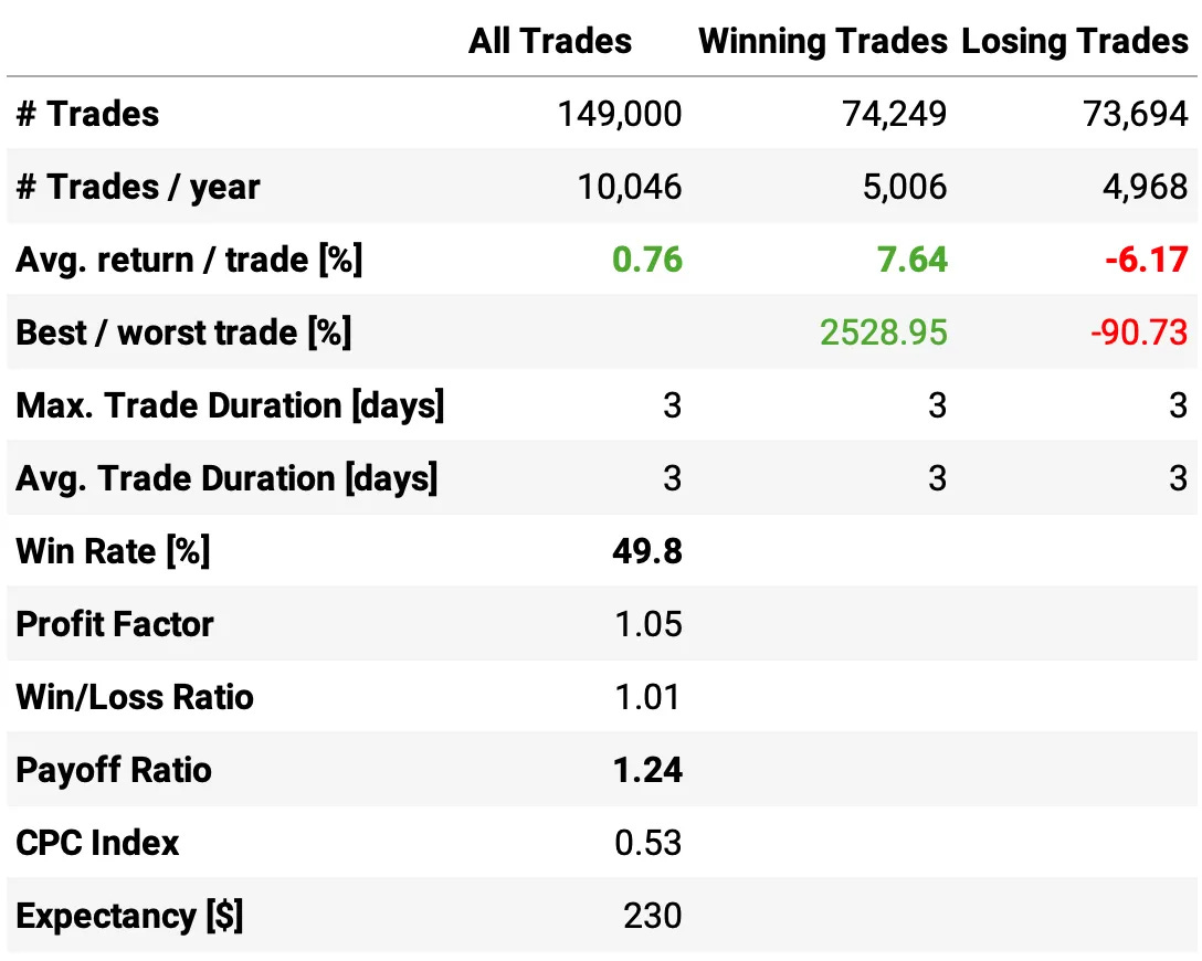
Here are the results of the first experiment:

Equity curve, drawdown curve, and annual returns for the first experiment

Summary of the backtest statistics

Summary of the backtest trades

Highlights:

• The first experiment delivered an impressive 21.7% annual return, ~2x the S&P 500 during the same period;

• The risk-adjusted return is 1.46, over twice the benchmark;

• The maximum drawdown is 21.8%, also better than the benchmark;

• The expected return/trade is +0.76%, with a win rate of 49.8% and a payoff ratio of 1.24.

Not bad for a first experiment. The most impressive result, in my opinion, is that this result is uncorrelated to the market: the correlation to S&P 500 daily returns is only 0.09.

Let's see if we can improve these results.

Reducing the number of positions

My first idea to improve the results is to reduce the number of positions: instead of 20 longs and 20 shorts every day, let's reduce it to 10. Additionally, let's relax the 3% maximum cap of any position, increasing it to 4%.

Equity curve, drawdown curve, and annual returns for the second experiment

Summary of the backtest statistics

Summary of the backtest trades

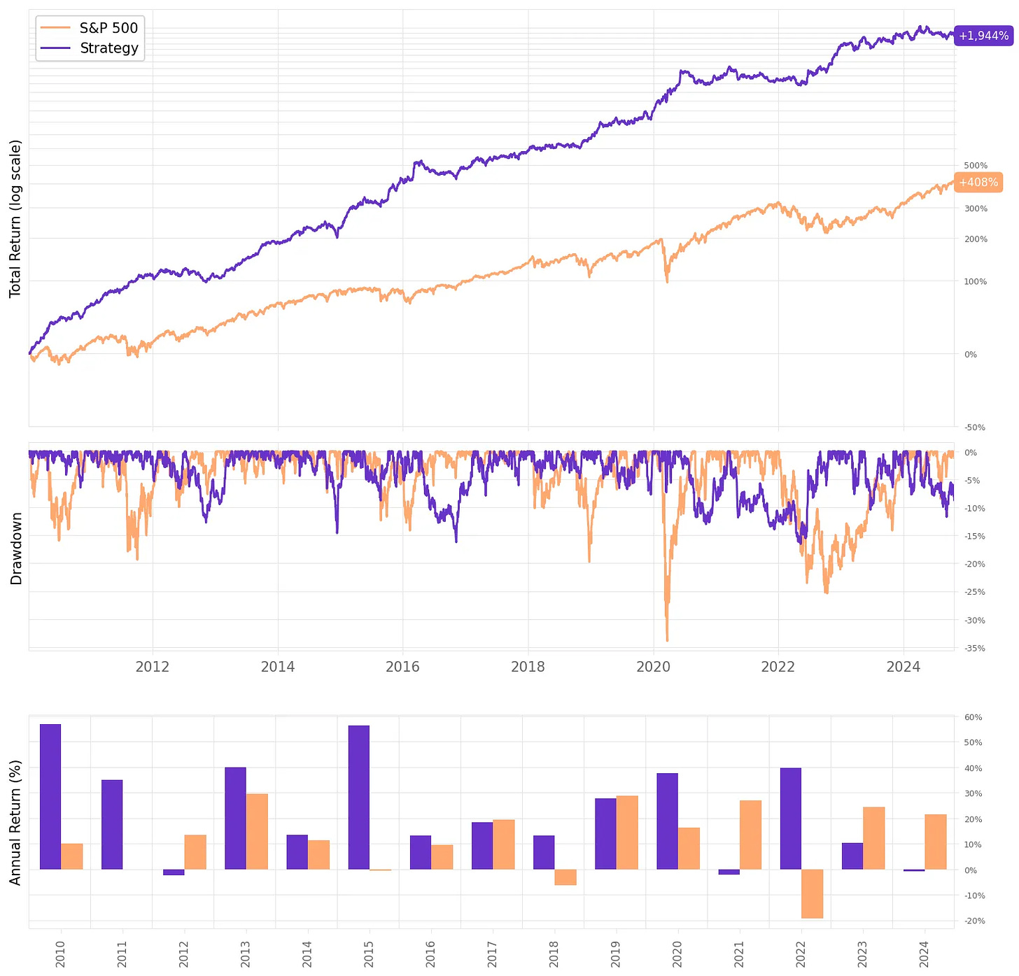
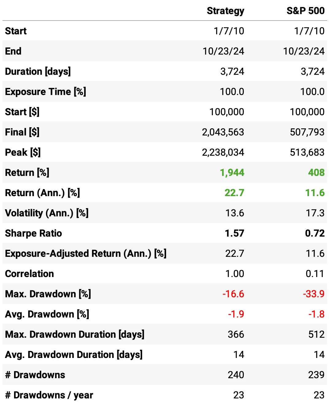
We were able to improve the results while cutting the number of trades by half. Here are the highlights:

• Annual return improved +1 ppt to 22.7%;

• Sharpe ratio also improved, now at 1.57;

• The maximum drawdown reduced to 16.6%, now less than half the benchmark;

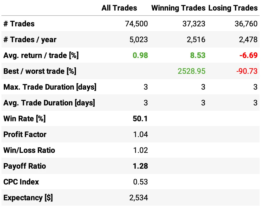
• The average return/trade improved to +0.98%, with an improvement in both the win ratio (now at 50.1%) and payoff ratio (now at 1.28).

The strategy continues with a low correlation to the market (0.11).

What else can we do to improve it?

Increasing the trade frequency

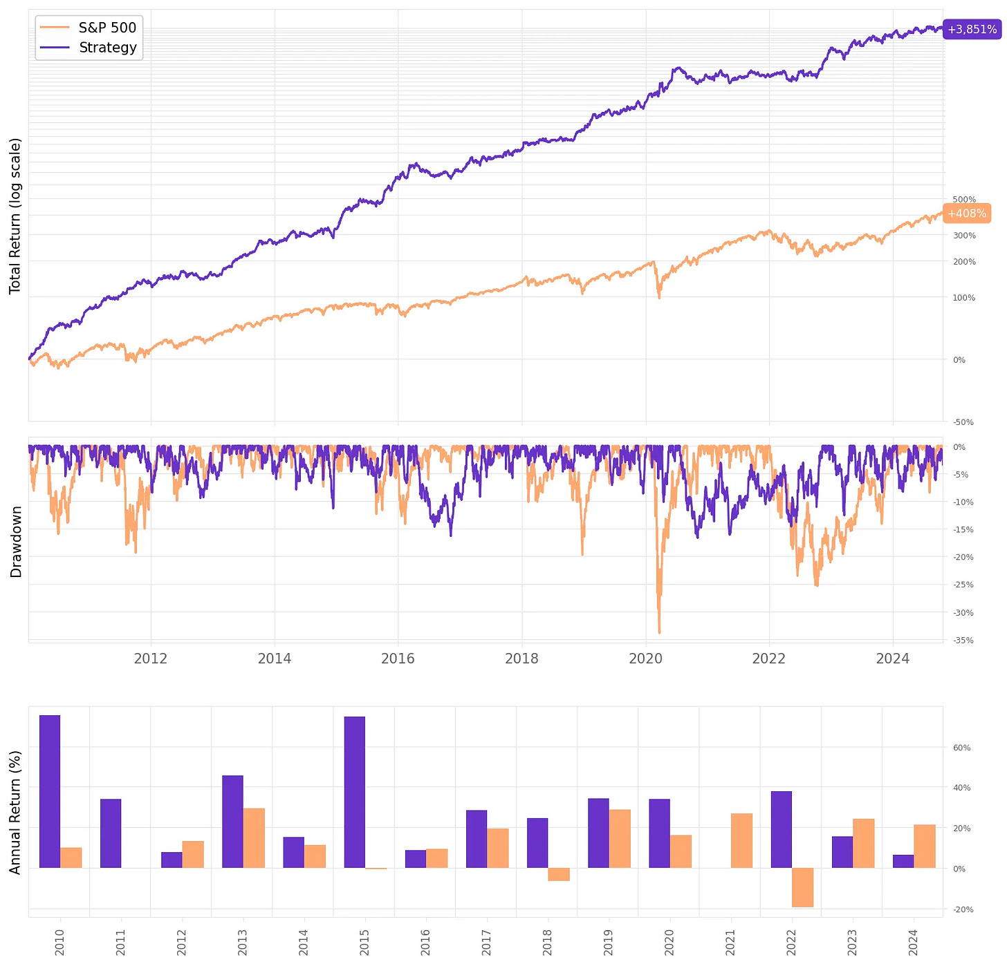
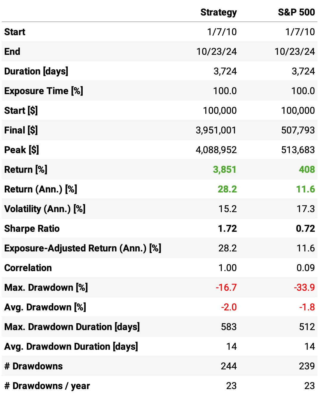
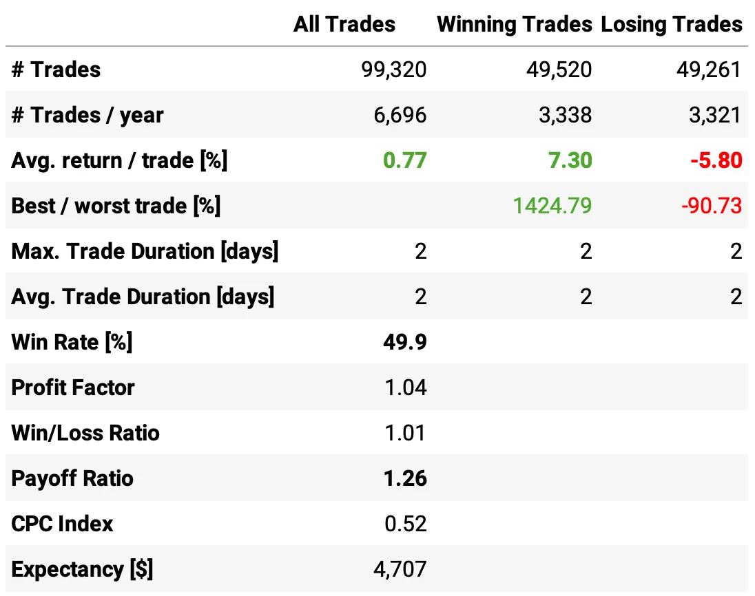
Now, instead of holding positions for 3 days, let's close it sooner, in 2 days. So, instead of splitting our capital into three portfolios, let's split it into 2. Let's see how increasing the frequency impacts the results:

Equity curve, drawdown curve, and annual returns for the third experiment

Summary of the backtest statistics

Summary of the backtest trades

So, much better results:

• The annual return had a significant improvement, now at 28.2%;

• The risk-adjusted return also improved, now at 1.72;

• The maximum drawdown remained at 16.7%.

Monthly and annual returns

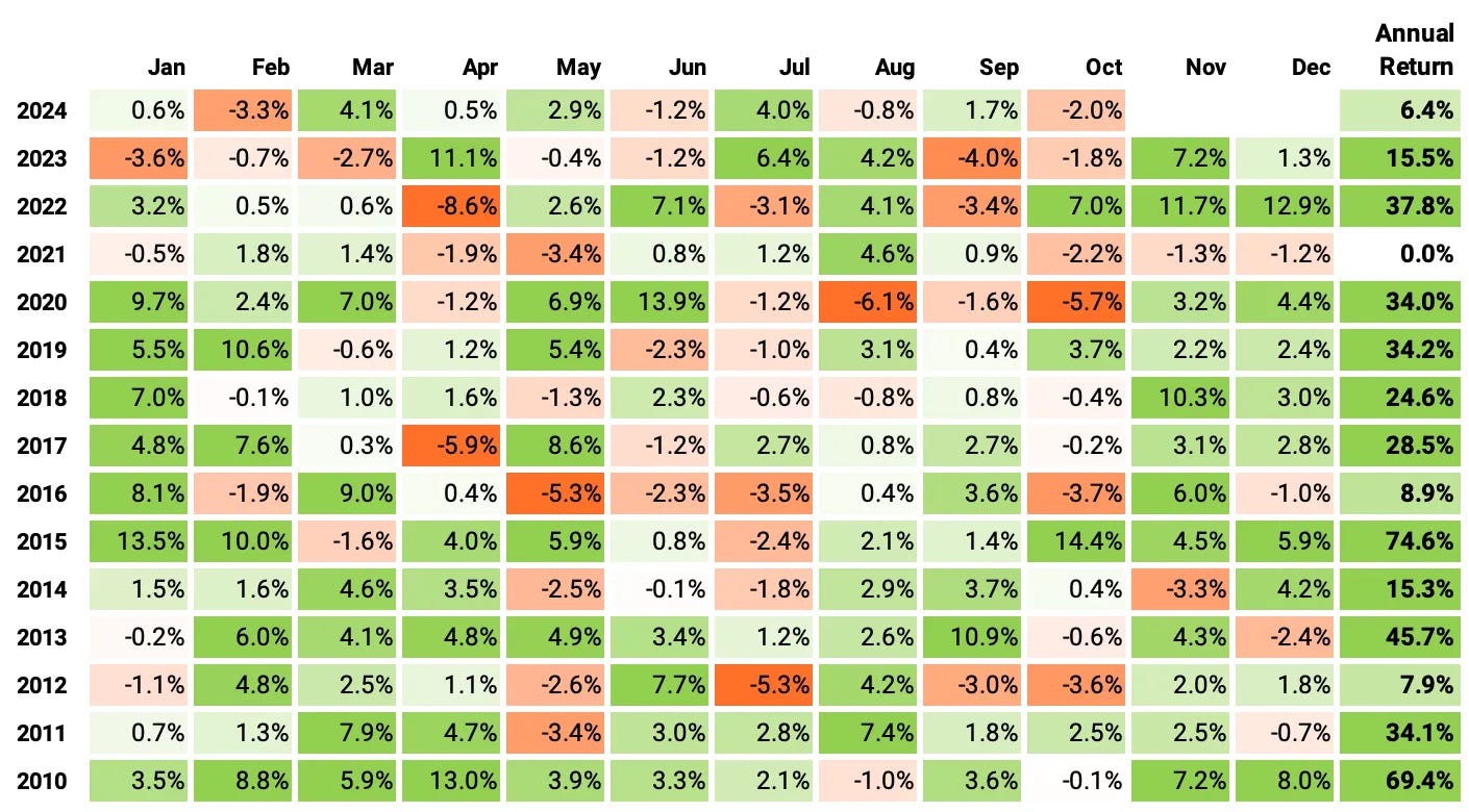
If we had traded this strategy since 2010:

• We would have had only positive years;

• We would have seen 66% of the months positive, with the best at +14.4% (Oct'15);

• We would have seen 34% of the months negative, with the worst at -8.6% (Apr'22);

• The longest positive streak would have been 18 months, from Aug'19 to Mar'20;

• The longest negative streak would have been 4 months, from Jul'20 to Oct'20.

How much of this performance is explained by common risk factors?

Now, let's use the Fama-French 3-Factor Model to analyze how much of the strategy's performance can be attributed to common risk factors like the market, size, and value. By running an OLS regression on the strategy's excess returns using the Fama-French factors, we can break down the sources of performance into:

1. Market Risk (Mkt-RF): The sensitivity of the portfolio to market movements, which reflects general market exposure.

2. Size (SMB): The sensitivity of the portfolio to the size factor, indicating whether it leans towards small or large-cap stocks.

3. Value (HML): The sensitivity to the value factor, showing whether it favors value or growth stocks.

We used the daily data from Kenneth French's website. Here are the results:

OLS Regression Results

Highlights:

• Alpha (0.0961): Statistically significant and positive, suggesting that the strategy has a daily excess return beyond what is explained by the three factors.

• Market Beta (0.0777): Statistically significant, a coefficient of 0.0777 indicates that for each 1% excess return in the market, the strategy's excess return increases by 0.0777%. So, our strategy is not very sensitive to the market, which was our intention.

• Size Beta (0.0316) and Value Beta (-0.0043): Neither is statistically significant, suggesting that exposure to small-cap or value stocks does not meaningfully impact the strategy's returns.

Also, we got an R-squared of 0.010 from the OLS regression results. An R-squared of 0.010 means that only 1% of the variation in daily excess returns is explained by the model. The low R-squared suggests that the model explains only a small portion of daily returns, which is what we want.

Final thoughts

As I mentioned in the introduction, this model is going into production, so yes, I am trading this system. Nevertheless, there are many improvements yet to be implemented:

• So far, the long and short positions are equally distributed across opportunities. We can try different weighting ideas;

• Throughout the simulation, there is cash sitting idle in the account (what is not required as margin for the short positions). We can invest this capital depending on the market regime, stacking the strategy's returns with other return streams;

• We can also apply the model to a narrower universe, such as the S&P Composite 1500 or even the S&P 500, and check the results.

Developing an idea like this took me a lot of time, especially debugging. But I'm glad it's now ready for forward testing.

I'd love to hear your thoughts about this approach. If you have any questions or comments, just reach out via Twitter or email.

Cheers!