Machine Learning and the Probability of Bouncing Back

Is it possible to get over 40% annual returns over the past 10 years trading an ML-based mean reversion model?

Woman with a Book. Pablo Picasso, 1932

The idea

“Learn the rules like a pro so you can break them like an artist.” Pablo Picasso.

Picasso painted “Woman with a Book,” one of his masterpieces, a few months before my grandmother was born. He was a legendary artist, a true master whose creativity and invention made him one of the most influential figures in modern art history. My grandmother has not achieved this level of notoriety—not even close. But she was also a true master. However, her craft was not the fine arts but fine cuisine.

When I was young, I used to watch her prepare her masterpieces. I loved to observe her work. Whenever we gathered the whole family, usually on special dates or holidays, she would prepare a special dish. And for that, she would get her cookbook.

Her cookbook was an old notebook full of handwritten recipes she had gathered throughout her entire life. In my view, the most amazing thing about her cookbook was that the recipes were not fully detailed with precise instructions. It had general instructions, the overall step-by-step, but not many details.

Her cookbook was of little to no value to me, as my abilities in the kitchen are pretty limited. But for a true master like her, it was a great asset. She was a pro, so she could understand the overall plan like no other and fill in the blanks with her creativity and decades of experience.

Later in life, I understood that the more details a recipe has (of any kind), the more it is designed for beginners. The more general a set of instructions is, the more it is intended for advanced users. My grandmother's cookbook made total sense.

This week, we will create a machine-learning model to predict the probability of a stock bouncing back once it deviates too far from the mean. I will describe the overall plan and how I came up with the model, but this time, I won't give all the details I've been doing so far. Here are the reasons why:

• This article is more geared toward advanced users, people with experience in Machine Learning. If I were to provide all the details a beginner would need to reproduce it, this article could end up being 10x larger. (Maybe someday I will write it.)

• As it is intended for more advanced users, I'm sure they will understand the overall step-by-step process and know how to fill in the blanks (as my grandmother did with her cookbook).

• I'm trading this model. One thing I learned from pros is that you don't share all the details of the systems you are actually trading.

Finally, in this article, we are going to break some rules. Many people, pros included, usually advise to “keep things as simple as possible.” This is generally good advice, which some people see as a rule never to be broken. However, as we are going to use a more sophisticated technique, we will leave the “as-simple-as-possible” realm. If you are uncomfortable with breaking this rule, no worries: just move to any other article (the vast majority are based on pretty simple rules… but not this one).

Some of my favorite books on machine learning

The ML model

So far, we have demonstrated several profitable mean reversion systems that consist of:

• A set of entry rules that, when triggered, tells our systems to get into a trade;

• A set of exit rules that, when triggered, tells the systems to get out of a trade;

• A universe of tradable securities from which the system selects the opportunities to trade.

In our last article, for example, we defined a mean reversion indicator (Quantitativo's Probability Indicator, or QPI) and set up systems that would enter trades whenever a stock from the S&P 500 crossed below 15. The system would then exit whenever its price closed above yesterday's high. Such a system works well.

This system would buy 100% of the times the entry signals were triggered.

But what if we could train a machine learning model to predict the probability of a stock bouncing back? Instead of buying 100% of the time, the model would look at some features from the stock (the QPI for different windows, RSI for different windows, rate of change for different windows, etc.) and then estimate its probability of bouncing back. Then, based on this estimated probability, the system would decide which stocks to trade.

Let's describe now how to create such a model in 3 steps:

1. The dataset and features;

2. The chosen algorithm;

3. The training process.

The dataset and features

I use Norgate data, a great survivorship-bias-free dataset. To collect data points, I settled on the Russell 3000 universe (current and past).

For features, I used:

• Rates of change for different windows (short, mid, and long terms, up to a year);

• RSIs for different windows;

• QPIs for different windows;

• IBS, Normalized ATR;

• Closing price distance to 200-day SMA;

• Turnover;

• Hurst exponent (I love this indicator and probably will write something especially for it in the future).

Pre-processing (extremely important):

• For features such as Turnover, I computed its relative value vs. past (time series) and relative value vs. all other stocks every single day (cross-sectional);

• For some other features, it makes sense only to compute its relative value vs. all other stocks every single day (cross-sectional);

• For others, it doesn't make sense to do any pre-processing computation;

• For features for which we computed cross-sectional relative value, it's usually a good idea to standardize.

Even if you have never created a model like this, if you think a bit, I think it will be fairly evident which features to apply the cross-sectional computation (and the standardization) to and which ones to leave as is.

For the target:

• For the target, we set 1 if the stock bounced back within 5 days (positive return) and 0 otherwise (further negative return).

Getting all Russell 3000 stocks from 1998 to today leads to over 17 million points.

Filtering only points that deviated from the mean above a certain threshold (QPI below 15, for instance) would reduce the dataset to approximately 1.3 million points. It's also important to filter for penny stocks (exclude all records when closing prices fall below $1), which leads us to 1.2 million data points.

I ended up with 16 features, so a matrix of 1.2 million rows and 17 columns to train our model.

The chosen algorithm

I formulated this problem as a binary classification problem. The trained model will try to predict whether a stock will revert to the mean (1) or not (0).

There are several possible algorithms. I've chosen XGBoost, of Extreme Gradient Boosting. Gradient Boosting is a machine learning technique that builds models sequentially, each new model focusing on correcting the errors made by the previous ones. It works by combining the strengths of weak models (often decision trees) to create a stronger, more accurate model.

Due to its performance and versatility, XGBoost has become a go-to tool for ML practitioners, especially in competitive machine learning. For more details about the algorithm, please check the XGBoost documentation.

The training process

To train the model, we will use the sliding window technique, with 15 years of lookback, retraining the model at the beginning of every year:

• 2014 model: trained with data from 1999 to 2013;

• 2015 model: trained with data from 2000 to 2014;

• 2016 model: trained with data from 2001 to 2015;

• 2017 model: trained with data from 2002 to 2016;

• 2018 model: trained with data from 2003 to 2017;

• 2019 model: trained with data from 2004 to 2018;

• 2020 model: trained with data from 2005 to 2019;

• 2021 model: trained with data from 2006 to 2020;

• 2022 model: trained with data from 2007 to 2021;

• 2023 model: trained with data from 2008 to 2022;

• 2024 model: trained with data from 2009 to 2023.

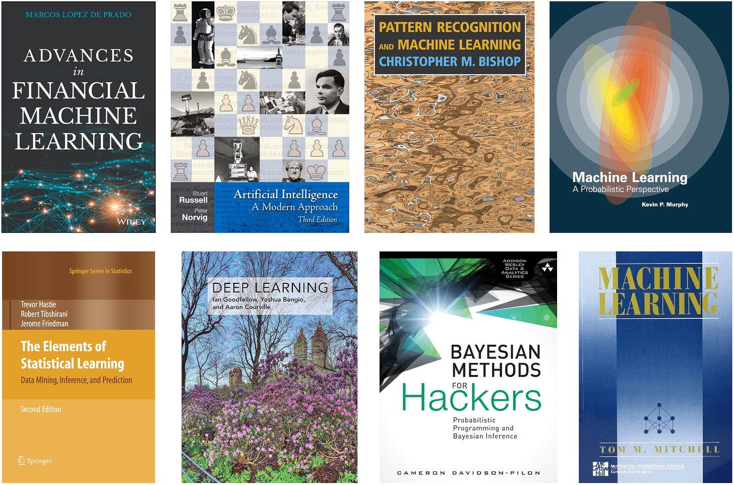
The book Advances in Financial Machine Learning 1st Edition by Marcos Lopez de Prado is a great read. It tackles all the details involved in the three steps I just described (and much more).

The edge

After training the model, the first question we want to answer is: what is the edge of using such a model?

Statistics of buying all events when the model tells the probability of a stock bouncing back is above 50% and holding for 5 days

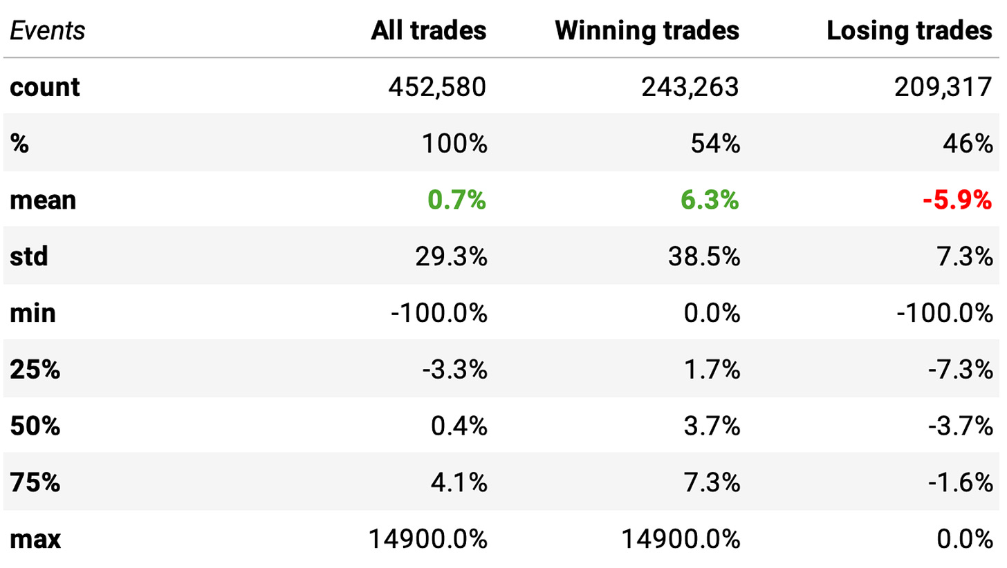
We see a positive expected return:

• We can expect a +0.7% return/trade;

• The win ratio is at 54%;

• There's a positive payoff ratio: the expected return on winning trades is +6.3%, vs -5.9% on losing trades.

But is this model better than just the simple rule of buying stocks whenever the QPI falls below 15 (like our previous article)? Let's check the stats and compare:

Statistics of buying all events when a stock drops its price, its QP drops below 15, and holding for 5 days

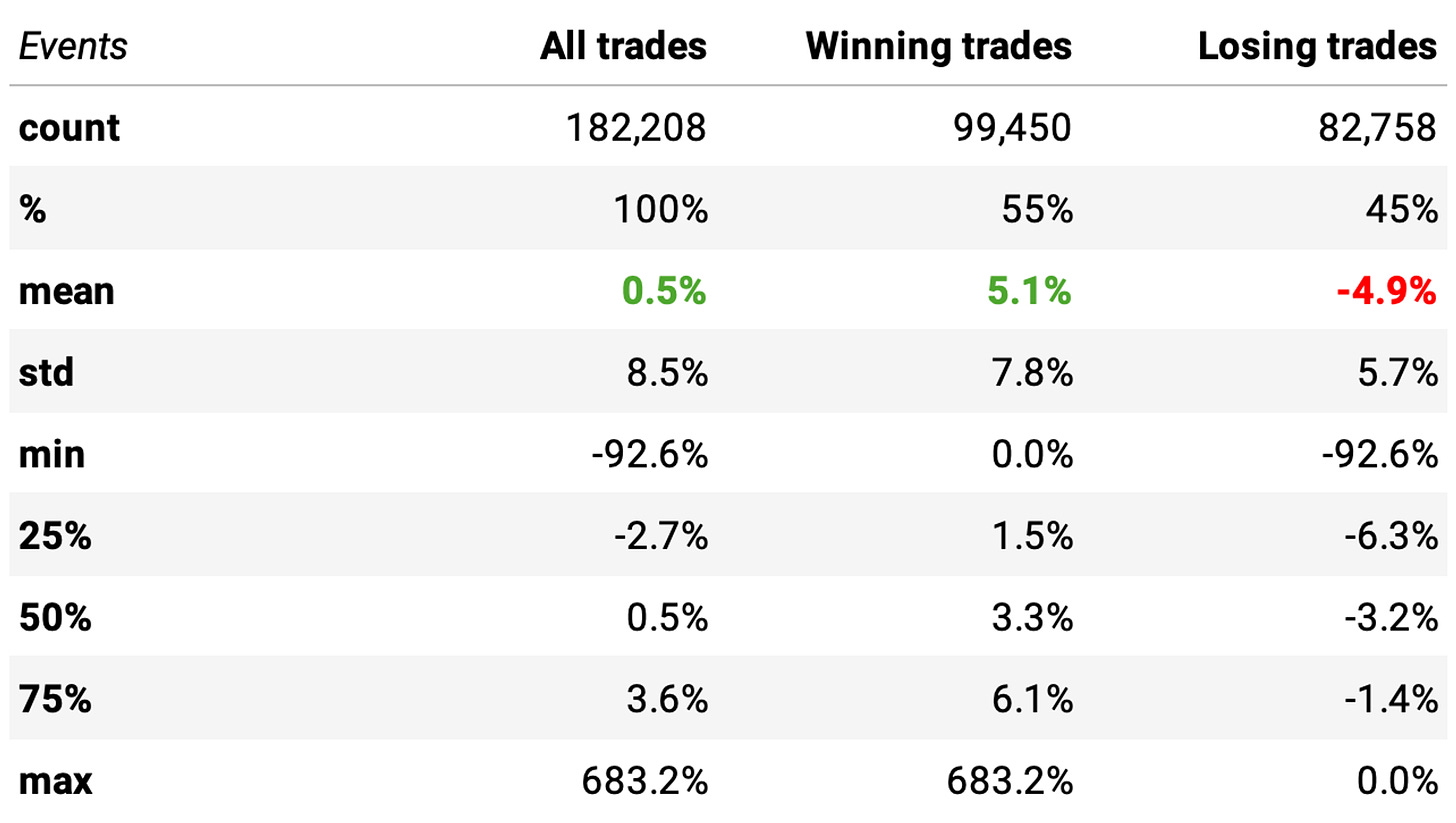
The expected return is pretty close.

Checking the P-value, we find 0.062, which is above 0.05. In other words, the means of the two distributions of returns are NOT significantly different. So, we do not have an edge. With the model as is, it's better to stick to the simple rules.

Tweaking the probability threshold

Before giving up, let's try the following change. The model we trained outputs the probability of a stock bouncing back. We are looking for the edge in buying all stocks whenever the model tells us the probability of a bounce back is above 50%.

What if we look for higher probabilities, like 60%? This means we will only act when the model is “more certain” about a trade to mean revert. Let's see the stats for a higher probability threshold (60%):

Statistics of buying all events when the model tells the probability of a stock bouncing back is above 60% and holding for 5 days

Wow! That's a significant improvement:

• The expected return/trade now is +1.6%, vs. the previous +0.7% (for 50% threshold);

• The win ratio is also higher, now at 56%;

• The payoff ratio is also better;

• The only downside is the number of events: as expected, with a lower probability threshold (50%), we would get more opportunities to trade (over 450k); now, with a higher bar (60%), we get about 1/4 of the opportunities (94k).

Most importantly, the P-value is now well below 0.05: the means of the two distributions are significantly different, so we have an edge.

The strategy

The strategy we will trade is simple. At the opening of every trading session:

• We will split our capital into 10 slots and buy stocks whose 3-day QPI from the previous day closed below 15, and the model we trained outputs a probability of bouncing back is above 60%;

• We will have no regime filter, as we included a feature that considers the distance between the closing price and the 200-day SMA;

• If there are more than 10 stocks in the universe with the entry signal triggered, we will sort them by the probability of bouncing back and prioritize the most probable moves;

• We will hold 10 positions maximum at any given moment.

To ensure we trade only liquid stocks:

• We won't trade penny stocks (whose closing price is below $1);

• We will only trade the stock if the allocated capital for the trade does not exceed 5% of the stock's median ADV of the past 3 months from the day in question.

Experiments

To have a baseline, let's start by only trading S&P 500 constituents (current & past, no selection bias):

Equity curve, drawdown curve, and annual returns for the first experiment

Summary of the backtest statistics

Summary of the backtest trades

These are not particularly great results. Annual return is just slightly better than the benchmark, while the maximum drawdown is higher. Sharpe ratio is barely better.

How can we improve it?

Trading the whole universe

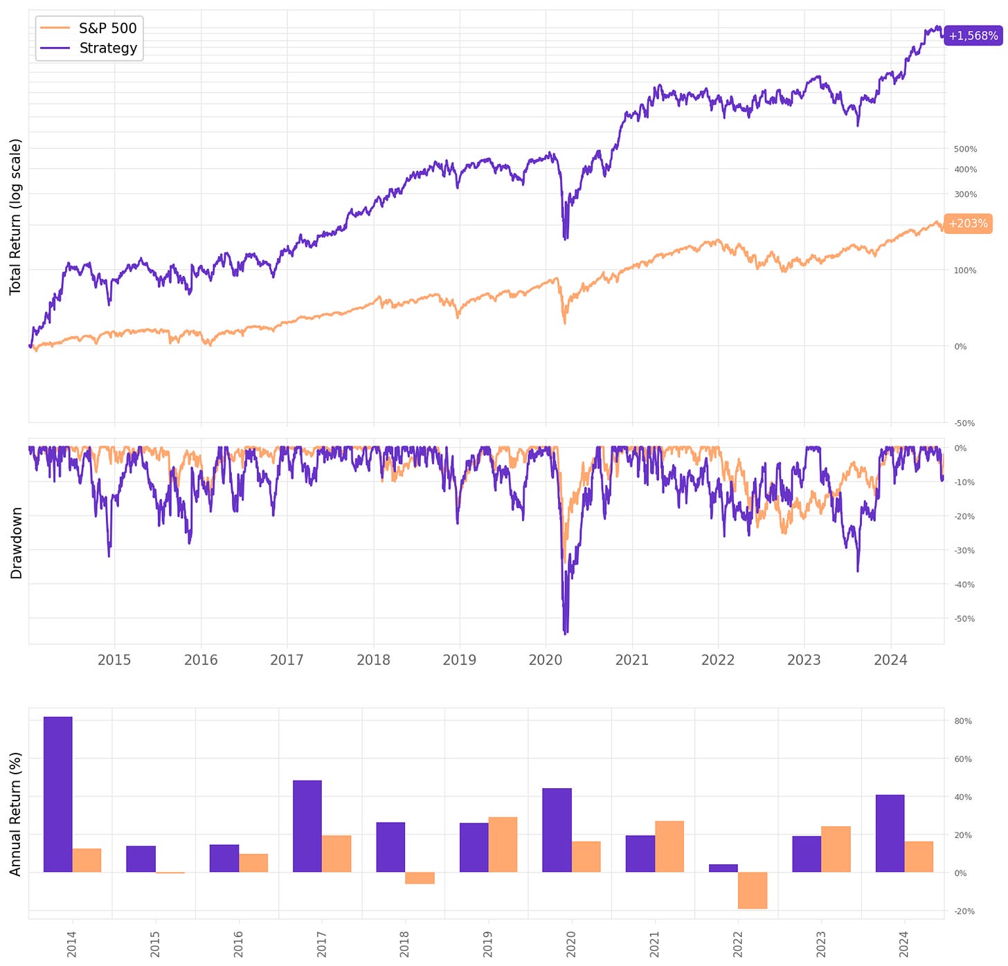
The first improvement is to trade the whole universe, which means all Russell 3000 stocks that meet our liquidity constraints. Here are the results:

Equity curve, drawdown curve, and annual returns for the second experiment

Summary of the backtest statistics

Summary of the backtest trades

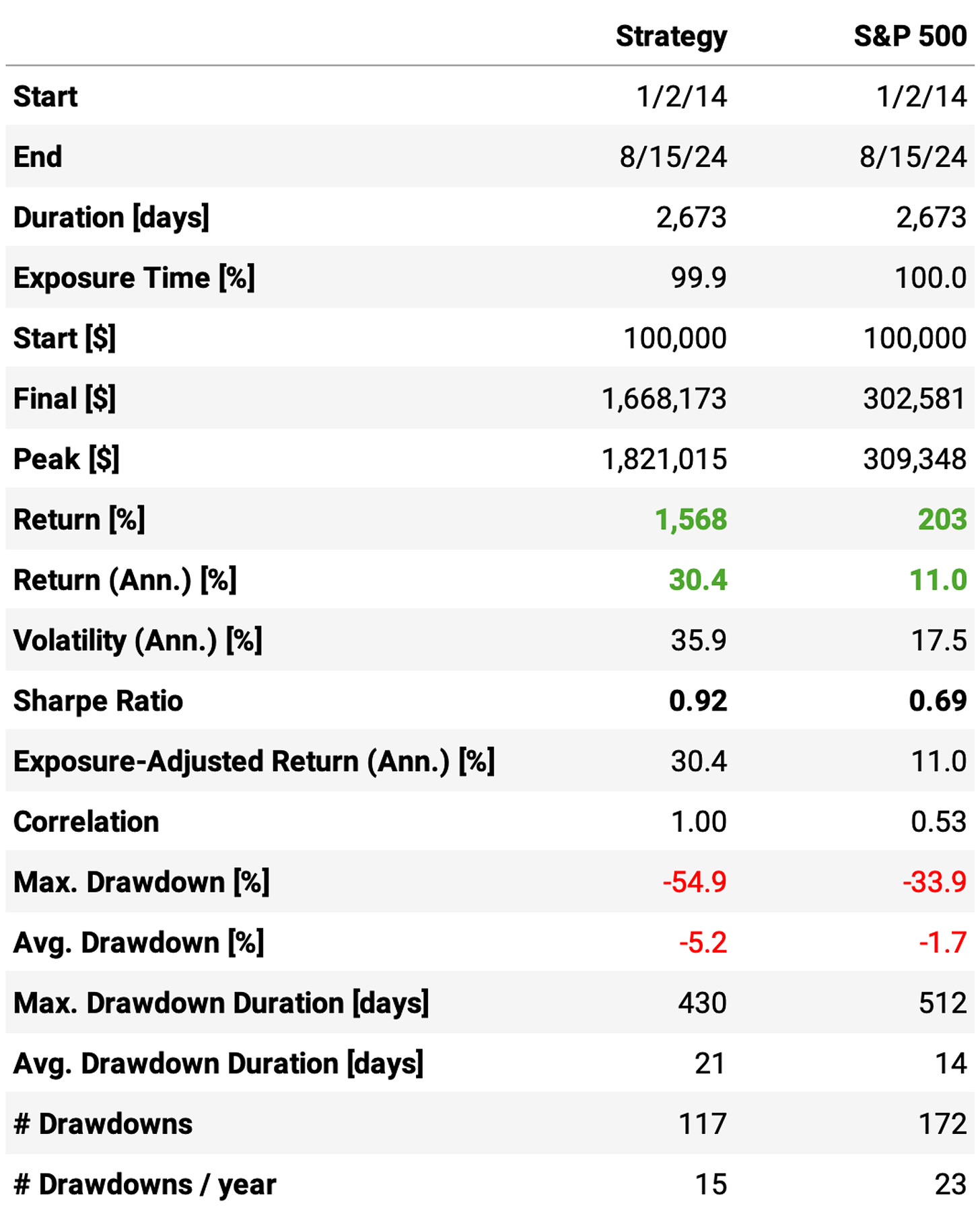
Much better results:

• Annual return now surpasses 30%, vs. 11% S&P 500;

• The Sharpe ratio is now at 0.92, vs. 0.69 the benchmark;

• However, the maximum drawdown is at 55%, vs. 34% the benchmark;

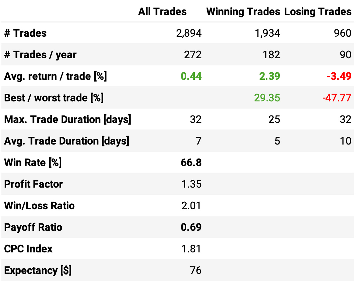
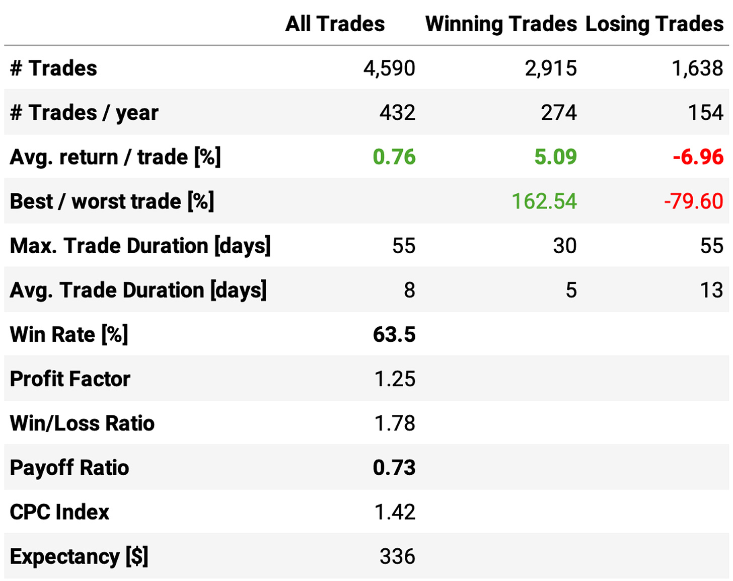
• The trade statistics are good: the average return per trade is +0.76%, with a win rate of 63.5% and a (not good) payoff ratio of 0.73.

Another interesting observation is that all years were positive. However, a maximum drawdown of over 50% would be too much for most traders. What can we do to try and improve that?

Testing stop-loss orders

Usually stop-loss orders do not work in mean reversion strategy. However, as we are using an innovative indicator to measure how far from the mean prices deviate, let's try them to improve the results.

In fact, we will try a combination of ideas to limit the losses:

• Stop loss orders: 5% below the entry price;

• Time limit: if the exit signal hasn't been triggered nor the stop loss, we will exit the trade after 6 days no matter what.

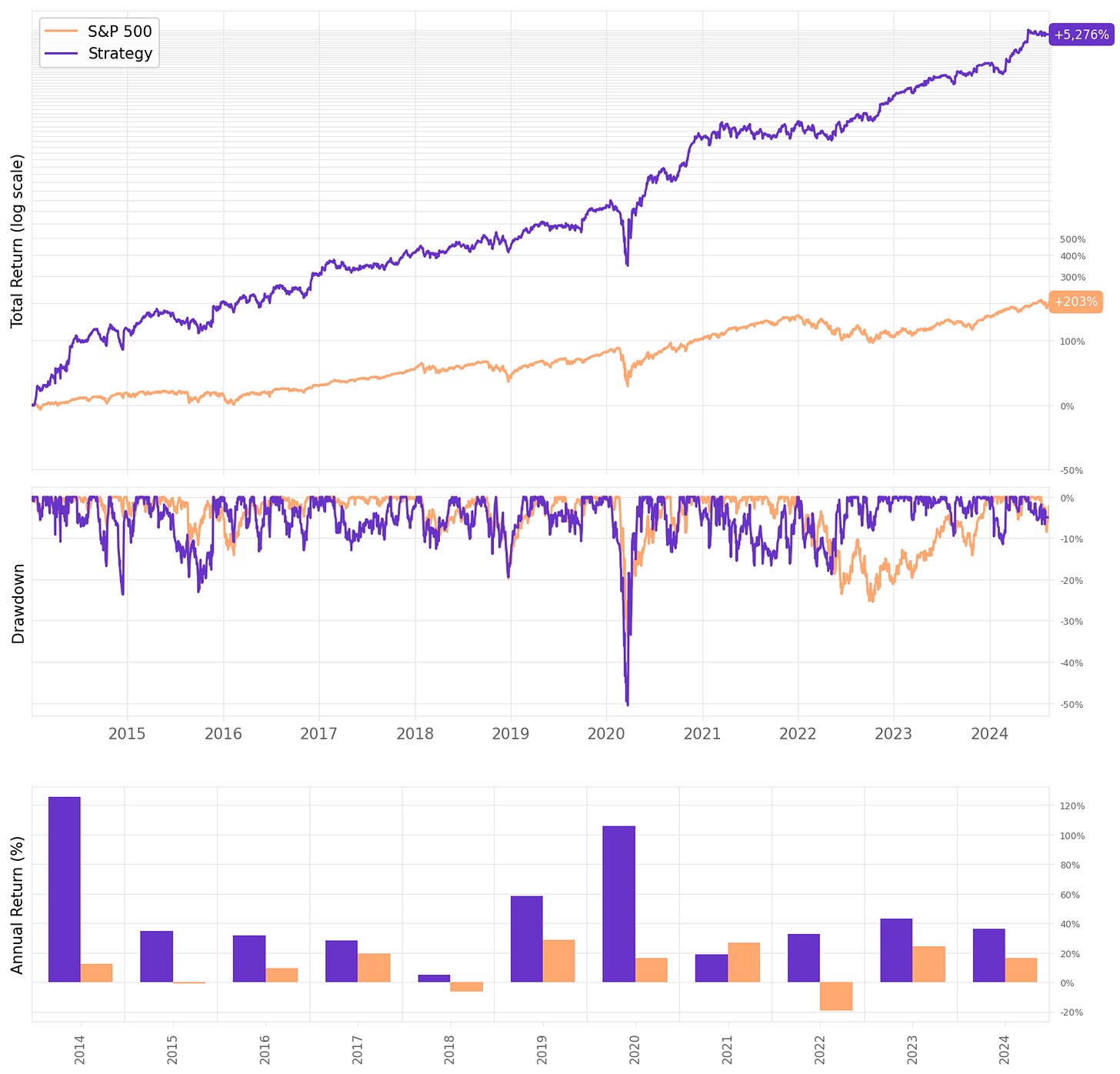
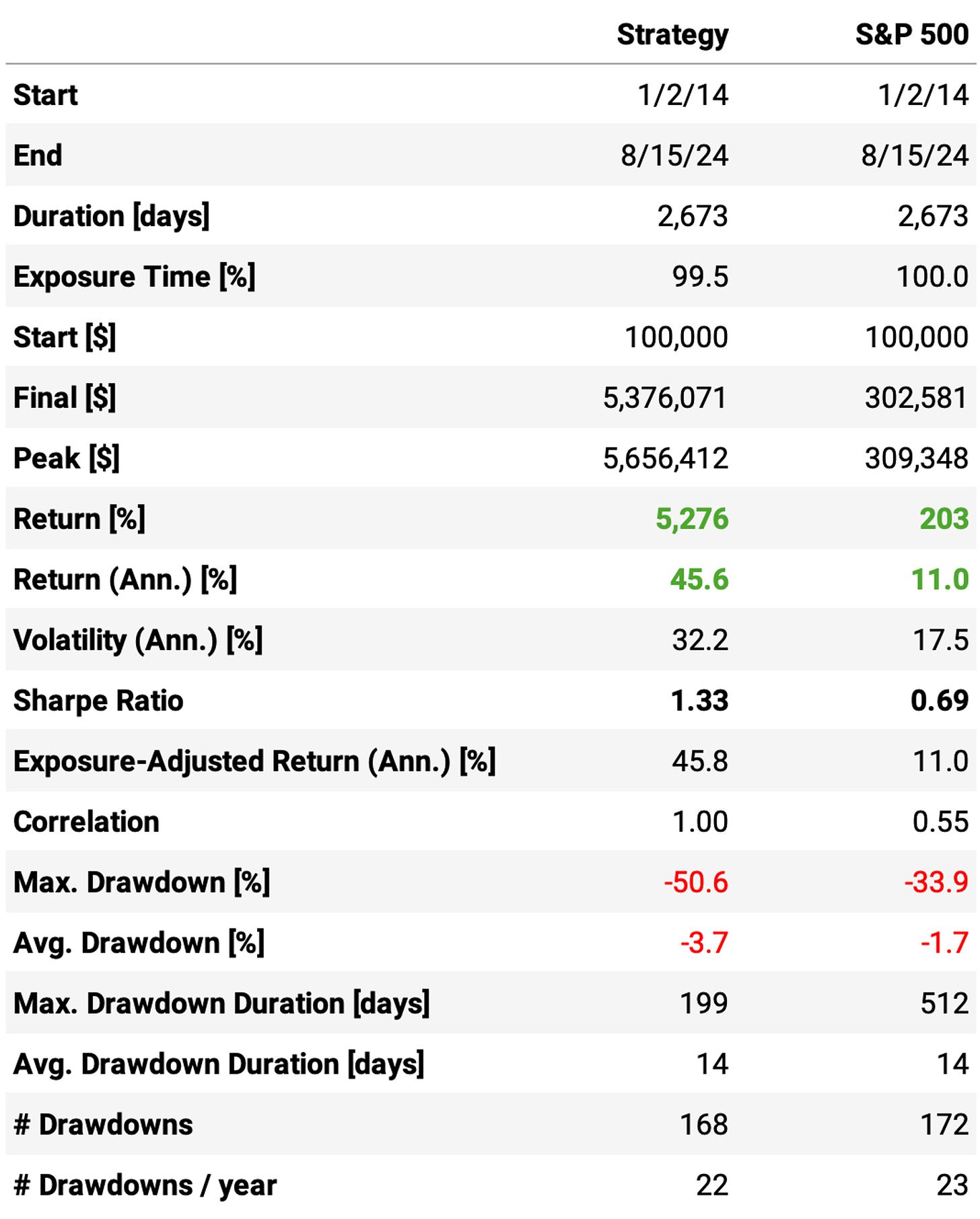
Here are the results:

Equity curve, drawdown curve, and annual returns for the final experiment

Summary of the backtest statistics

Summary of the backtest trades

These results are not bad! Highlights:

• Annual return reaches 45.6%, over 4x the benchmark;

• Sharpe ratio is now at 1.33, almost twice of S&P 500's;

• However, maximum drawdown continues pretty high at 50%;

• Implementing the stop loss and the time limit reduced the win rate to 60%;

• However, the expected return/trade remained about the same, at +0.73%;

• But most importantly, the payoff ratio improved from 0.73 to 0.86.

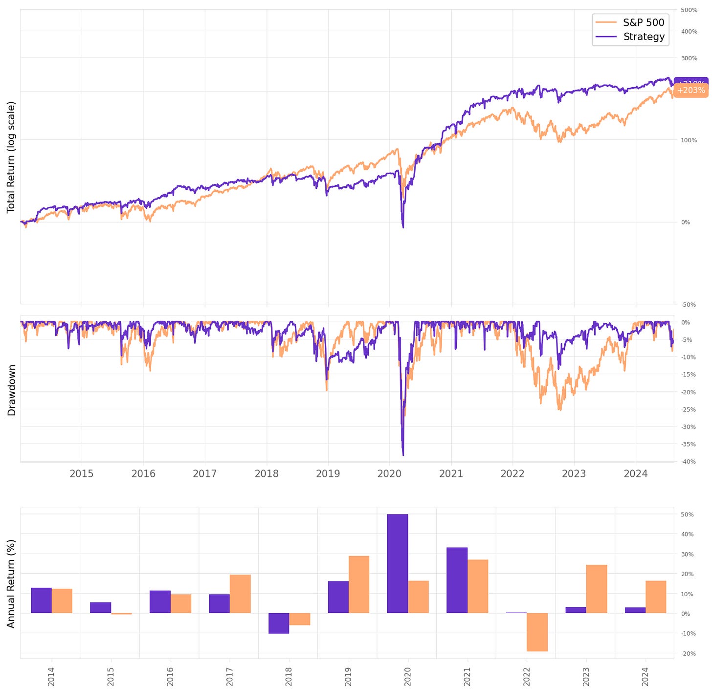
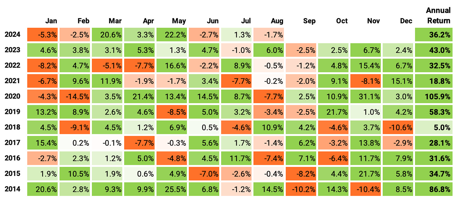
Let's look at the monthly and annual returns:

Monthly and annual returns

If we had traded this strategy since 2014:

• We would have had only positive years, no down years;

• We would have seen 64% of the months positive, with the best at +31.1% (Nov’20);

• We would have seen 36% of the months negative, with the worst at -14.5% (Feb'20, COVID);

• The longest positive streak would have been 9 months, from Oct'22 to Jun'23;

• The longest negative streak would have been 4 months, from Jun'15 to Sep'15.

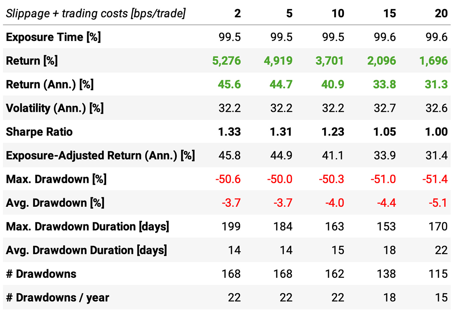
Trading costs

The 2-basis points assumption for slippage + trading costs might not hold anymore now that we are trading stocks beyond what is present in either the S&P 500 or NASDAQ-100. So, let's see how different levels of trading costs impact the results:

Impact of trading costs

Final thoughts

The ideas I shared today might resonate differently with each person. For those who followed the reasoning, are able to implement this idea, and have questions, just send them and I will try to answer all, as usual.

For those who followed the reasoning and would like to learn all the details about how to implement an idea like this one, I will try to find time to create in-depth material explaining every step of this recipe. It will take some time.

As I broke some rules in this article, I understand people may criticize, some constructively and some destructively. I will respond to all constructive comments; the others, I will ignore.

There are several improvements to be made in this system:

• We only trained a model to recognize price-drop patterns and predict the probability of upward mean reversions, so, a natural next step is to train a model to be used in the short leg;

• The system currently allocates the capital across all opportunities equally, not taking into consideration the probability of mean reverting; so, another area of improvement would be to adjust the positions according to the probability output from the model;

• Excluding COVID, all drawdowns are about 20% or lower; nevertheless, we could try to add a regime filter to avoid events like that.

I'd love to hear your thoughts about this approach. If you have any questions or comments, just reach out via Twitter or email.

Cheers!