

Learning to Rank
A market-neutral strategy that delivers 18% annual returns with a 13% max drawdown


The idea
“Give me a firm place to stand and a lever, and I can move the Earth.” Archimedes.
Archimedes, the brilliant Greek mathematician and engineer, was so fascinated by levers that he claimed he could move the Earth with one. His deep understanding of mechanics made him a legend, from designing war machines to discovering buoyancy while lounging in a bathtub. Just as he used levers to amplify force, money managers use leverage to amplify market exposure—turning small amounts of capital into powerful positions. When applied wisely, it can be a game-changer.
This week, we will implement the paper Building Cross-Sectional Systematic Strategies By Learning to Rank by Daniel Poh, Bryan Lim, Stefan Zohren, and Stephen Roberts. Published in 2021, the paper explores how machine learning techniques, particularly learning-to-rank algorithms, can enhance the construction of systematic trading strategies. Let me start by saying why I chose this particular paper.
Over the past few months, I’ve had the opportunity to learn more about first-loss funds. Among the funds I spoke with, market-neutral strategies are the preferred choice. With that in mind, I’ve been exploring ideas that align with this approach, and the Learning to Rank paper immediately caught my attention. Its unique methodology sparked my curiosity, making it a perfect candidate for deeper analysis.
As always, replicating the exact results from a research paper proved challenging—but I managed to get promising outcomes worth sharing. One key factor made all the difference: leverage. That’s when Archimedes came to mind. I carefully applied leverage while keeping gross exposure within levels that would meet first-loss funds’ risk guidelines. But I’m getting ahead of myself—let’s take it step by step.
Here's the plan for today:
Summarize the paper – a quick overview of its core ideas;
Explain our implementation – highlighting both similarities and differences;
Replicate the backtest results – seeing how well they hold up;
Propose improvements – exploring ways to refine the strategy.
Unlike last week, I won’t be sharing the code for this paper here. This project is more complex; a full breakdown would make the post too long. Instead, I’ll include it in the course I’m developing, where I’ll provide my complete multi-asset Python backtester, my analysis & visualization modules, 3–4 fully implemented strategies, and execution code for forward testing and live trading. I’ve already written about 30% and should have it wrapped up in the next few weeks.
I’ve been using the survey below to understand better what types of strategies our community is most interested in. If you have 60 seconds, I’d love to hear your input:
Now, to the strategy!
Paper summary
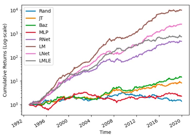
The paper introduces Learning to Rank (LTR) as a novel approach to enhance cross-sectional systematic trading strategies, particularly momentum-based strategies. Traditional ranking methods, such as sorting past returns or using regression-based forecasts, often fail to optimize ranking accuracy, leading to suboptimal portfolio performance. LTR, widely used in search engines and recommendation systems, improves ranking precision by learning pairwise and listwise relationships between assets. The study applies LTR techniques to a cross-sectional momentum strategy and demonstrates that Sharpe Ratios can be tripled compared to traditional methods. This provides a flexible, generalizable framework for improving asset selection in systematic trading.
The paper explores three LTR categories:
Pointwise methods (inferior ranking accuracy);
Pairwise methods (RankNet, LambdaMART);
Listwise methods (ListNet, ListMLE).
LTR learns the relative rankings of assets instead of just their expected returns.
LambdaMART performs best across profitability, ranking accuracy, and risk metrics: we will focus on this algorithm. Please check the paper for a full review of all the different methods.
Here is the summary of the main details:
Universe Selection:
Uses CRSP data (1980-2019) for NYSE-listed stocks.
Includes only actively traded stocks above $1 with at least one year of price history.
Portfolio Construction Framework:
Features
Compute asset scores using past returns, volatility-normalized indicators, and momentum signals.
Score Ranking
Apply LambdaMART to rank stocks based on future expected performance.
Security Selection
Go long the top decile and short the bottom decile based on rankings.
Volatility Scaling
Normalize position sizes based on ex-ante monthly volatility, targeting 15% annualized volatility.
Re-Training & Rebalancing:
Model re-training: Every 5 years (parameters are fixed for the next 5 years).
Portfolio rebalancing: Monthly (on the last trading day of each month).
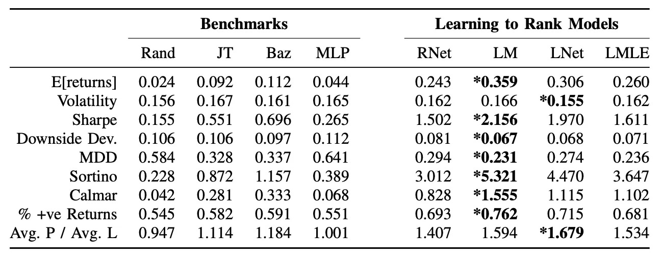
Performance Results:
LTR methods significantly outperform traditional ranking techniques.
Sharpe Ratios triple compared to classical cross-sectional momentum strategies.
LambdaMART delivers the best returns and ranking accuracy.
Lower drawdowns and downside risk compared to regression-based approaches.
Key Takeaways:
Learning to Rank enhances cross-sectional strategies by improving asset selection.
LambdaMART is the most effective method, balancing accuracy and efficiency.
The framework is modular, allowing incorporation of alternative features beyond momentum.
Potential future improvements include model ensembling and higher-frequency applications.
The strategy - our implementation
We did some important changes in implementation. Here are the main differences and similarities:
Universe Selection:
Instead of CRSP data, we used Norgate data
We used Russell 3000 Current & Past stocks, taking care only to include stocks when they were part of the index
Portfolio Construction Framework:
Features:
The 21 features used to train the model are implemented exactly as described in the paper: 6 features are past returns (raw and normalized, different windows), and 15 are momentum based (different windows)
Target and model:
Next month returns are used to rank the stocks
LambdaMART models this ranking and learns to predict it
Security Selection:
We replicated the 10 deciles as described in the paper
Additionally, we experimented with 20, 30, 40, 50, 60 quantiles as well
Volatility Scaling/leverage:
My experiments with volatility target didn't work as reported in the paper; so, I used equal weights for all long & short positions
However, I did apply leverage: instead of 100% gross exposure, I used 150% gross exposure
Re-Training & Rebalancing:
Model re-training: Every year instead of every 5 years as proposed in the paper. At every year, the model was retrained using past 15 years of data.
Portfolio rebalancing: Monthly (on the first trading day of each month instead of the last as proposed in the paper)
I haven't performed any optimization whatsoever, as I believe that would lead to overfitting. In fact, to prevent overfitting, I did the following changes in XGBoost's default parameters:
✅ Max depth reduction from 6 to 5 → Limits tree complexity, reducing variance and making the model less prone to memorizing noise.
✅ Learning rate reduction from 0.3 to 0.1 → Slows down learning, ensuring smoother updates and better generalization. Helps prevent overfitting to short-term patterns in ranking.
✅ Number of trees increase from 100 to 200 → Compensates for the lower learning rate, allowing the model to gradually improve without aggressive updates.
These details were omitted in the paper, yet they are essential for a successful implementation. Quantitative research papers often leave out such specifics, making it our responsibility to bridge the gaps.
Finally, here are my trading cost assumptions: I assumed 10 bps per trade, covering slippage, commissions, and borrowing fees, applied uniformly across all stocks. The paper did not account for trading costs, arguing that the strategy rebalances monthly, which helps minimize their impact compared to higher-frequency approaches. For backtesting, I believe this assumption should suffice. If the results look promising, the next logical step would be forward testing, which provides a more detailed view of real-world trading costs.
The edge
After training the model, the first question we want to answer is: what is the edge of using such a model?
To analyze that, we:
Compute the prediction for every stock in the universe for every day since 2006;
Compute the realized future returns for every stock;
Aggregate by decile and annualize returns.
Here's what we found:
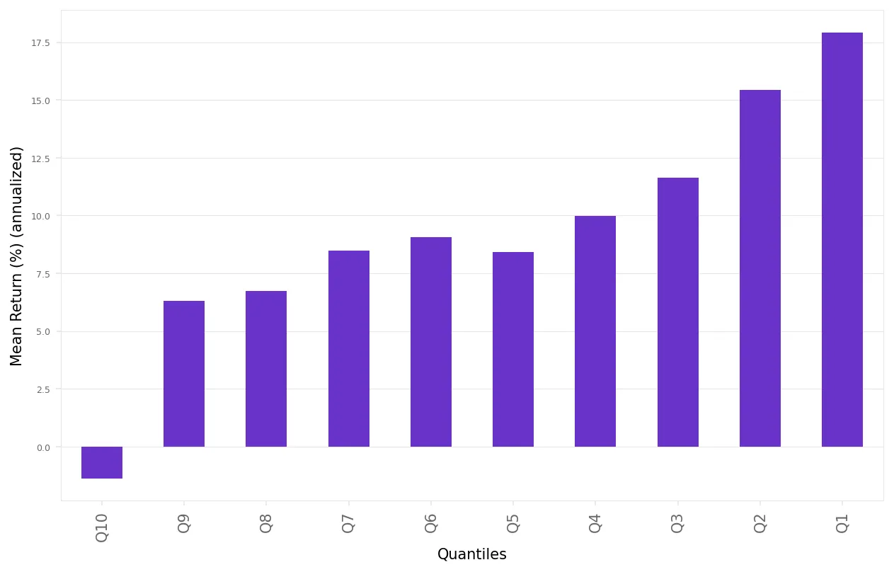
The results align with our expectations:
The top 10% of stocks (1st decile) generate the highest returns.
The bottom 10% of stocks (10th decile) produce the lowest returns, which are negative.
This confirms the foundation for constructing a long-short portfolio.
Now, let's see the experiments.
Experiments
Here are the results of the first experiment:

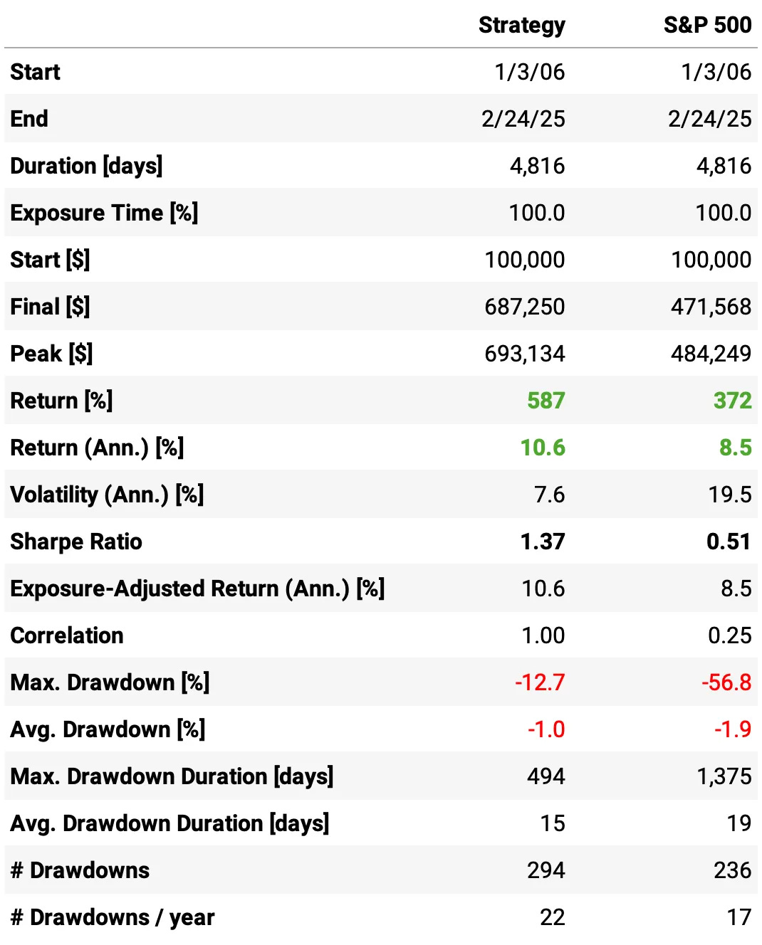
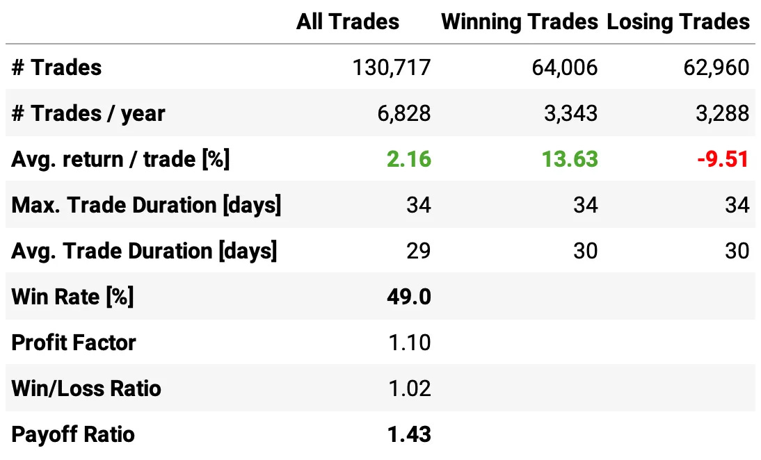
Highlights:
The first experiment delivered a 10.6% annual return, slightly above S&P 500 during the same period;
The risk-adjusted return is 1.37, over twice the benchmark;
The maximum drawdown is 12.7%, much better than the benchmark;
The expected return/trade is +2.16%, with a win rate of 49.0% and a payoff ratio of 1.43.
Not bad for a first experiment, especially for a strategy that executes monthly rebalances. Let's see now how to improve these results.
Number of stocks in each portfolio
Looking at the previous table, we notice a high number of trades per year, despite the portfolio being rebalanced monthly. Why is that?
The reason is excessive diversification due to using 10 quantiles. Since our universe consists of Russell 3000 stocks, each long portfolio, on average, holds 300 stocks, and each short portfolio holds the same.
To create more concentrated portfolios, we can increase the number of quantiles, reducing the number of stocks selected per bucket. Let's analyze how this parameter affects the results:
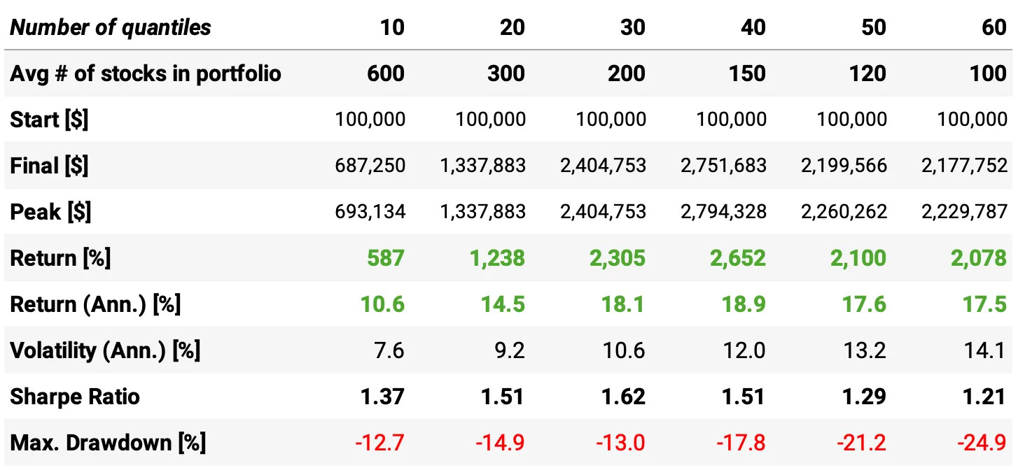
Looking at the results, we can draw interesting conclusions:
Higher concentration improves returns but increases volatility and drawdowns:
Return (Ann.) rises from 10.6% (10 quantiles) to 18.9% (40 quantiles)
Volatility increases from 7.6% to 14.1%
Max drawdown worsens from -12.7% to -24.9%
Optimal trade-off around 30-40 quantiles:
Best Sharpe Ratio (1.62) at 30 quantiles
Highest return (2,652%) at 40 quantiles
Beyond 40 quantiles, Sharpe Ratio declines due to higher volatility and drawdowns
Too many quantiles (50-60) degrade risk-adjusted returns
Sharpe Ratio drops to 1.21 at 60 quantiles
Drawdowns exceed -20%
A moderate number of quantiles (30-40) provides the best balance between return and risk. Let's settle in 30 quantiles and see its results:
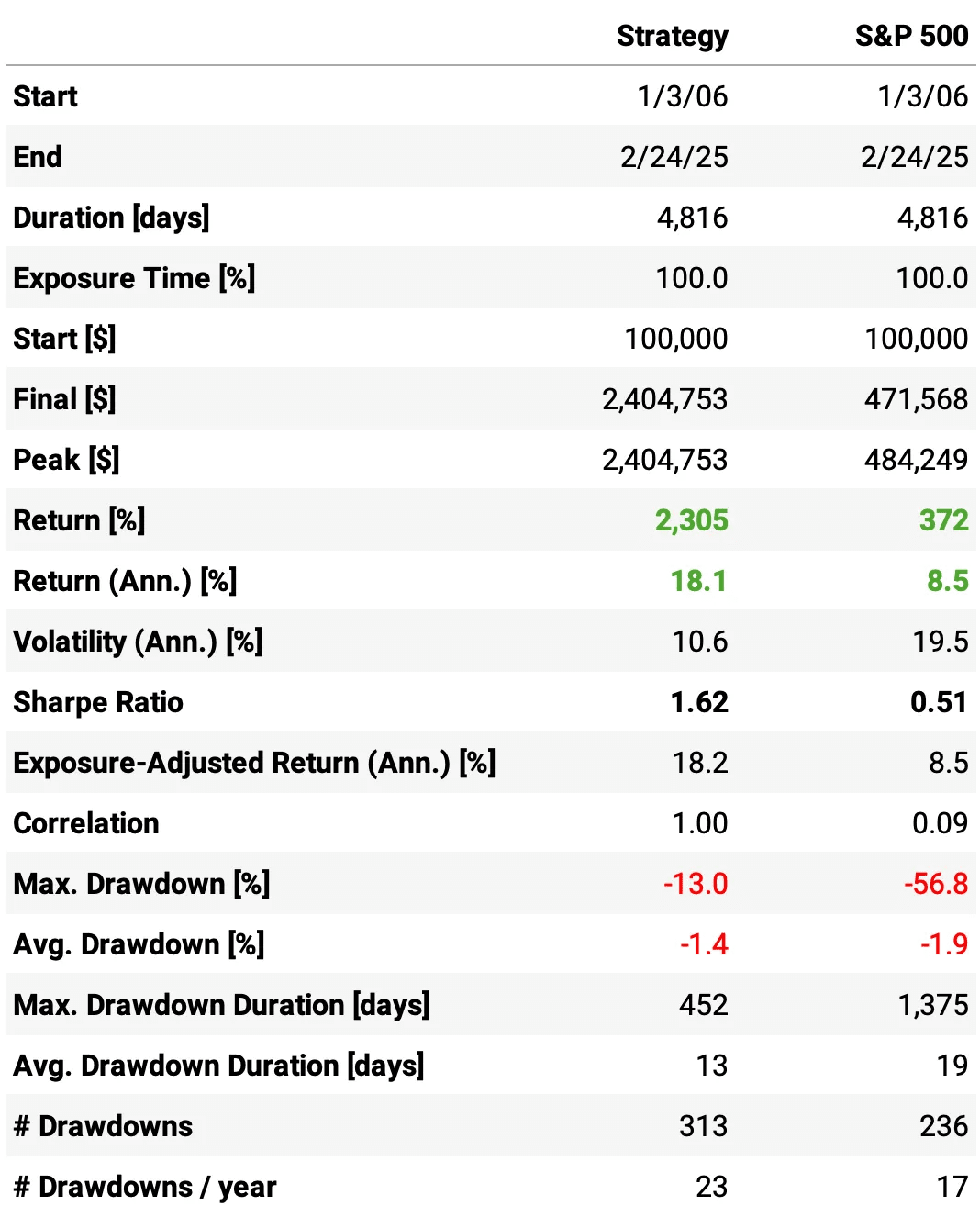
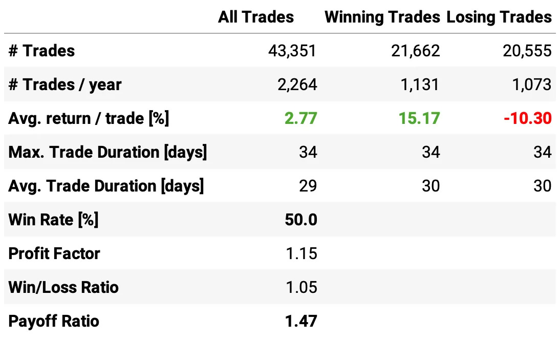
Highlights:
The strategy achieves an 18.1% annual return, more than double the 8.5% of the S&P 500.
The Sharpe Ratio is 1.62, significantly higher than 0.51 for the benchmark
Volatility is 10.6%, much lower than the 19.5% of the S&P 500
Maximum drawdown is -13.0%, far better than -56.8%
Correlation with the S&P 500 is only 0.09, indicating diversification benefits
The expected return/trade is +2.77%, with a win rate of 50.0% and a payoff ratio of 1.47, a nice improvement vs. the first experiment
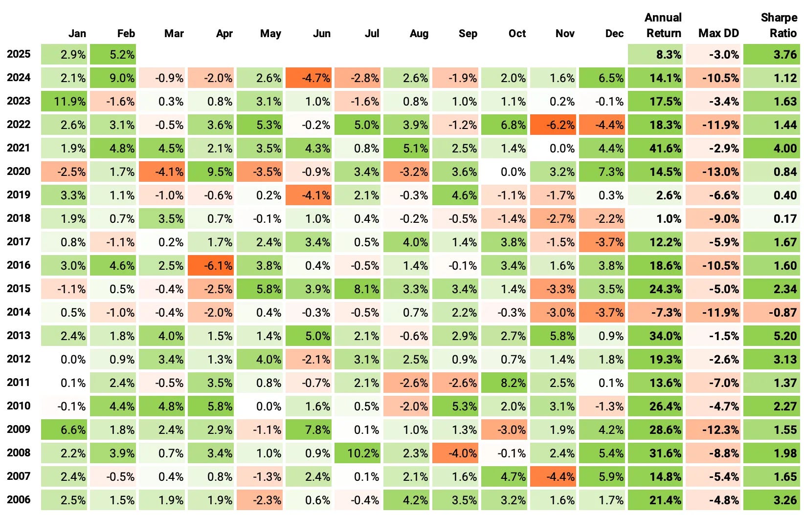
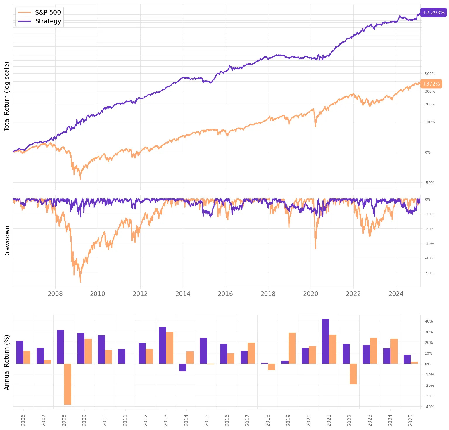
If we had traded this strategy since 2006:
We would have had only one negative year;
We would have seen 70% of the months positive, with the best at +11.9% (Jan'23);
We would have seen 30% of the months negative, with the worst at -6.2% (Nov'22);
The longest positive streak would have been 16 months, from Nov'20 to Feb'22;
The longest negative streak would have been 5 months, from Aug'18 to Dec'18.
How much of this performance is driven by common risk factors?
To better understand what’s driving the strategy’s returns, we apply the Fama-French 3-Factor Model to analyze its exposure to well-known risk factors: market, size, and value. By performing an OLS regression on the strategy’s excess returns using these factors, we can break down its performance into:
Market Risk (Mkt-RF): Measures how sensitive the strategy is to overall market movements, capturing broad market exposure.
Size (SMB): Evaluates whether the portfolio has a tilt toward smaller or larger stocks.
Value (HML): Determines whether the strategy favors value stocks or growth stocks.
For this analysis, we used daily factor data from Kenneth French’s website. Here are the results:
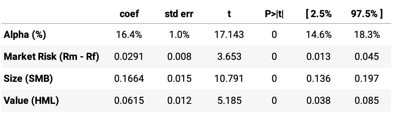
Highlights:
Alpha (16.4%): Statistically significant and positive, indicating that the strategy delivers 16.4% annualized excess returns beyond what is explained by the three factors. This suggests strong idiosyncratic performance independent of common risk premia.
Market Beta (0.0291): Statistically significant, meaning the strategy has some exposure to market risk, but the low coefficient suggests that it is not highly sensitive to market movements, aligning with the goal of a market-neutral approach.
Size Beta (0.1664): Highly significant, indicating a tilt toward small-cap stocks. This suggests that a meaningful portion of the strategy's returns is influenced by the size factor.
Value Beta (0.0615): Statistically significant, showing that the strategy leans toward value stocks, though the effect is smaller than the size factor.
Final thoughts
LTR-based strategies offer a fresh perspective on asset ranking, improving trade selection and overall performance. While this research-backed approach is promising, its practical implementation requires careful adaptation to account for trading constraints, costs, and execution dynamics. With further refinements, this could become a robust foundation for a market-neutral strategy suitable for institutional portfolios.
The results we obtained, while promising, were inferior to those reported in the paper—our Sharpe Ratio of 1.62 falls short of the 2.16 achieved in the original study. This discrepancy is largely explained by differences in the dataset, parameter choices, and the inclusion of trading costs. We used Norgate data with Russell 3000 stocks, retrained the model annually instead of every five years, and applied a 10 bps trading cost assumption, all of which contributed to a more conservative outcome. Despite these differences, the strategy still demonstrates strong performance and risk-adjusted returns, reinforcing its potential.
There are many improvement ideas:
Use model ensembling to combine multiple LTR models and improve ranking robustness.
Experiment with feature selection techniques to refine the most predictive signals.
Apply LTR techniques to higher-frequency data (e.g., intraday or order-book features).
Investigate shorter rebalancing periods (e.g., weekly or daily) to optimize market responsiveness.
Replace equal-weighted position sizing with dynamic volatility-based allocation.
Integrate alternative data sources such as earnings transcripts, analyst ratings, or news sentiment to enhance ranking predictions and improve signal quality.
I'd love to hear your thoughts about this approach. If you have any questions or comments, just reach out via Twitter or email.
Cheers!
Hi!
Would be great to see how your strategies would do if executed on close vs open (what you seem to do systematically). I think a lot of the edge would go away but there would also be less slippage.
I would love to see this as future post!
Keep up the good work
Nice write up,
I am trying to replicate but one thing I am not sure about is how you go about labeling the data using future returns. rank:pairwise requires 0 or positive integers so using raw future returns wouldn't work. What method would you suggest labeling the data here?