Intraday Momentum for ES and NQ
A system that delivered +1.5 Sharpe ratio over the past 15 years
The idea
"If I have seen further, it is by standing on the shoulders of giants.” Sir Isaac Newton.
First of all, Happy New Year! When I started Quantitativo a few months ago, I could never expect to gather such an amazing group of like-minded people in such a short time. Your enthusiasm, curiosity, and engagement have made this journey incredibly rewarding and inspiring.
Reflecting on the many, many messages I've received since I published the first article, the number 1 request has been to share more details and possibly the source code. I am working on that - more news on that front soon.
Starting this year, I decided to write about my implementation of popular papers in the field. So, starting with this article, I will implement a paper every once in a while, reproduce the results achieved by the research, and then try to contribute by adding original ideas on top of what has been built. The idea is to stand on the shoulders of giants, as Sir Isaac Newton put it.
The first paper for which I will share my implementation and some potential improvements is titled 'Beat the Market: An Effective Intraday Momentum Strategy for S&P500 ETF,' by Carlo Zarattini, Andrew Aziz, and Andrea Barbon. The reasons for this particular choice are:
Many readers asked about my take on this work;
I am particularly interested in developing more trend-following/momentum strategies.
So, here's our plan:
First, we will quickly summarize the strategy as described in the paper;
Then, we will evaluate if the edge is statistically significant;
Then, we will replicate the backtest results presented in the paper;
Finally, we will propose some improvements.
Strategy summary
The strategy's core idea is to exploits intraday trends caused by demand/supply imbalances, avoiding periods of market noise. In a nutshell:
Key Elements:
The authors define a Noise Area using past intraday price movements over 14 days;
Trades are initiated when the price moves outside this area, indicating significant demand/supply imbalance;
Positions are closed either at the market close or when the price reverses back into the Noise Area.
Trailing Stops:
Enhanced risk management includes dynamic stops based on the Noise Area boundaries or VWAP (Volume-Weighted Average Price).
Risk Adjustment:
Positions are adjusted based on recent market volatility, targeting consistent risk exposure.
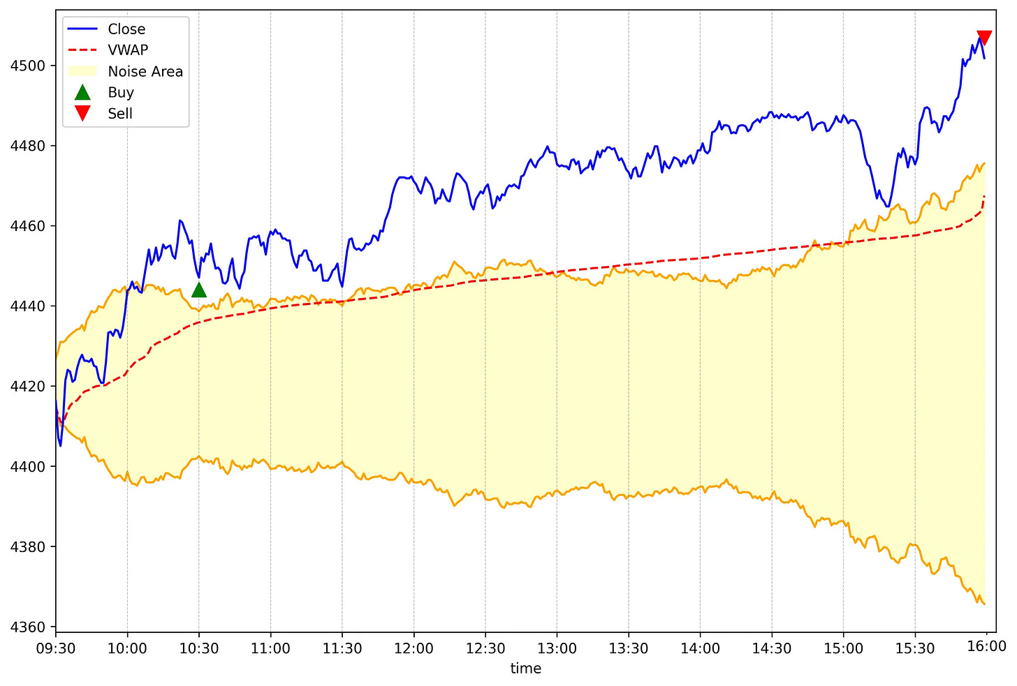
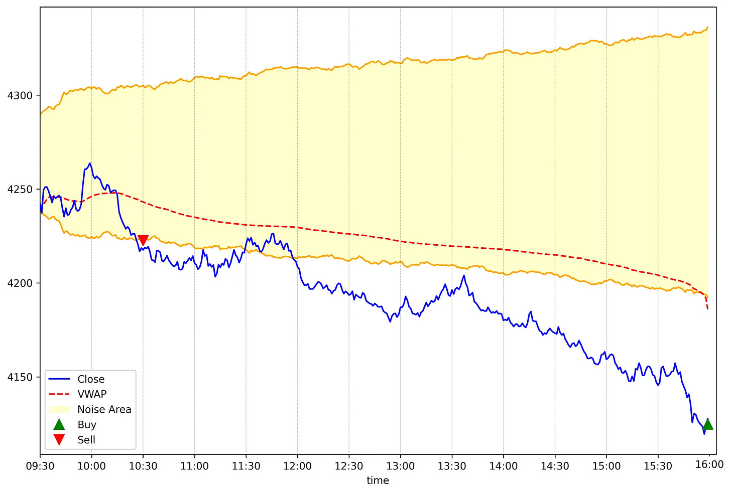
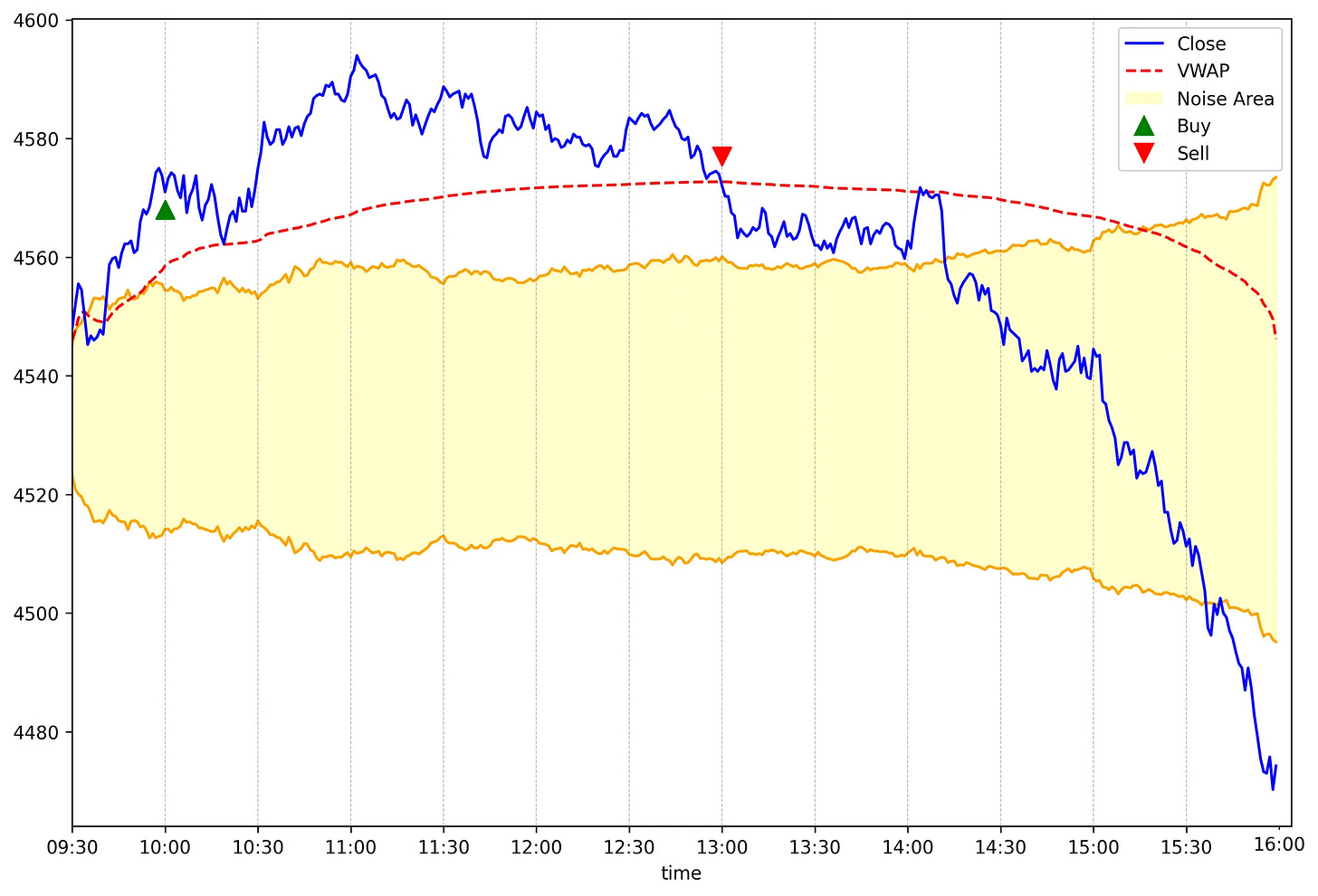
Here's some trade examples:
For more details on how to implement the rules, please check the paper.
The edge
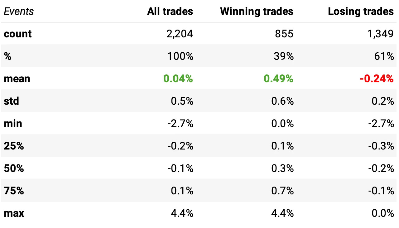
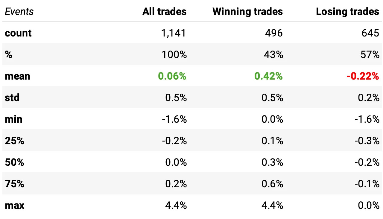
Let's start the analysis by evaluating what would have happened if we had took all long & short opportunities according to the rules above.
Important: for the analysis, we used Databento's minute data since 2010. In all numbers, we considered 1 tick in slippage, IBKR's fixed commissions and exchange fees.
Highlights:
Overall, taking all trade opportunities has a positive expected return per trade (after costs) of +4 bps (+6 bps longs, +3 bps shorts)
The win ratio is 39% (43% longs, 34% shorts)
The payoff ratio is approximately 2:1 (shorts over 2:1)
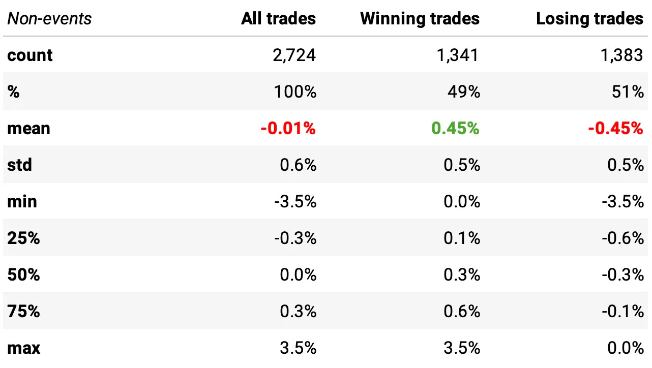
Now, let's check the overall stats of non-events: what would have happened if we had traded all days when the entry signal was not triggered (long and short)?
As expected, trading non-events would be a coin-flip. But most importantly, the P-value is well below 0.05: the means of the two distributions are significantly different. So, we have an edge.
Now, let's see how this strategy backtests from 2010 to today.
Experiments
Our first experiment is the implementation of the paper, but with the following changes:
Instead of using SPY ETF, we use ES futures contract (always the most liquid contract)
Instead of considering the trading costs as presented in the paper, we used $0.85/contract in commissions + $1.40/contract in fees (per transaction, i.e., we multiply by 2 for every trade), and 0.25 tick in slippage in every transaction (i.e., 0.5 tick per trade)
All the other rules are kept as presented in the paper. Important: we apply the 2% target daily market volatility, capping the leverage at 4x as the authors did.
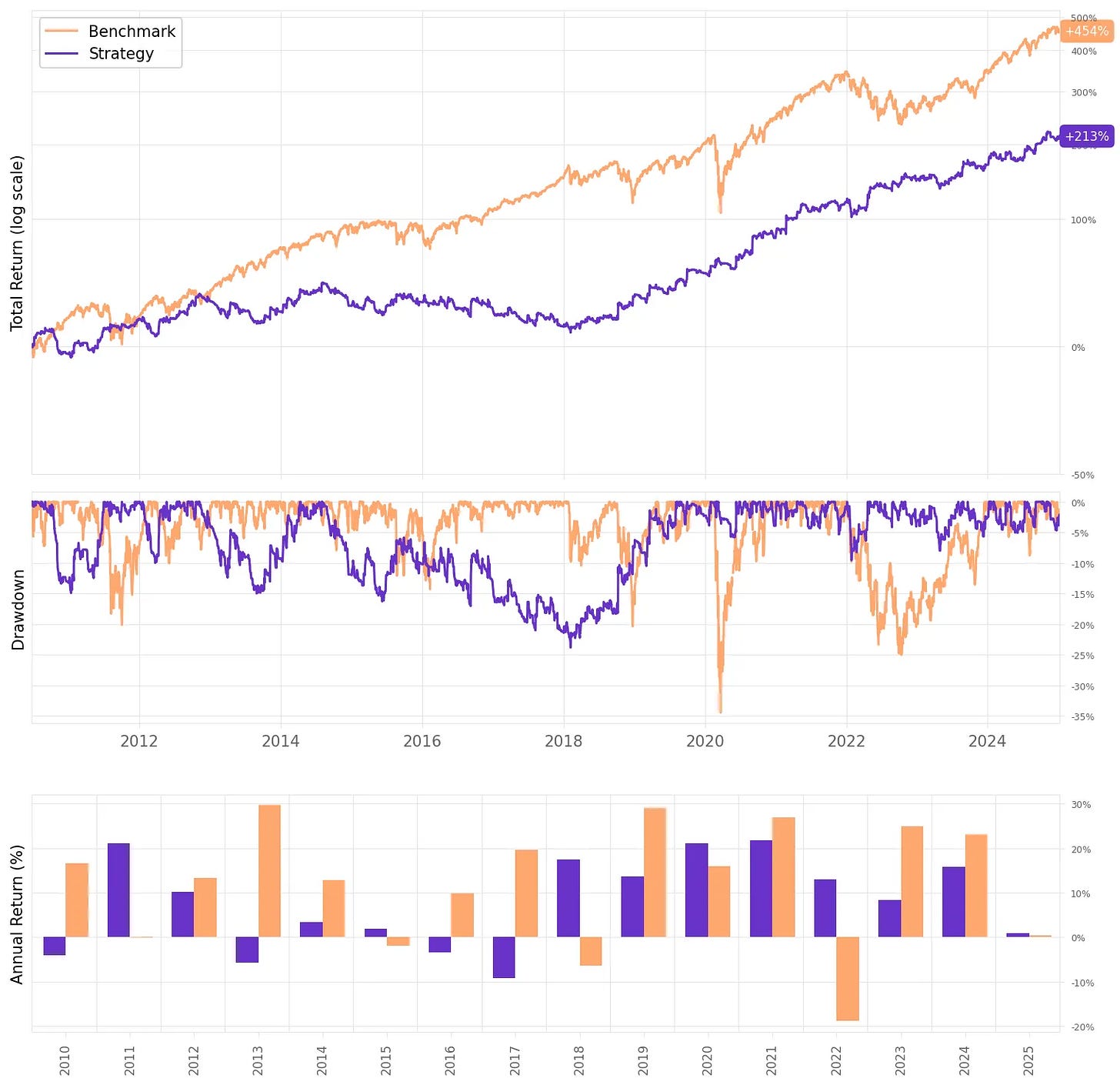
Here are the first results:
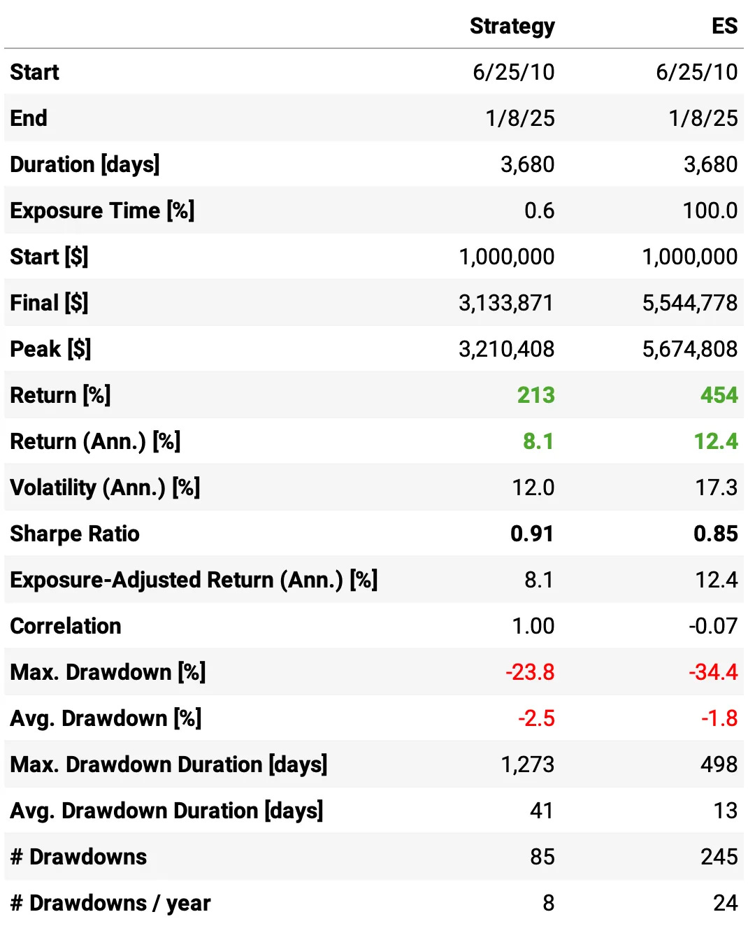
The results are somewhat inferior than what was achieved by the authors in the paper:
Annual return is +8.1% vs 12.4% the benchmark;
Sharpe ratio is 0.91, slightly above benchmark;
Max drawdown is at 24% vs. 34% NQ long only;
The expected return/trade is +2 bps, with a win rate of 36% and a good payoff ratio of 2.09.
Two reasons explain the difference:
In the paper, the authors start the backtest in 2007. This makes a significant difference, as 2008 is a great year for the strategy, and a very negative year for the market;
Also, slippage assumptions cause a significant impact. The lower the slippage assumption, the better the results. However, I don't think it's realistic to assume less than 0.5 tick/trade, which is already optimistic.
The strategy is basically flat from 2010 to 2017, and then starts working from 2018 on.
Let's see how we can improve these results.
Adjusting the lookback and adding leverage
To compute the noisy area, which is critical to define the entries and stop losses, the paper uses a lookback window of 14 days. The first adjustment we will implement to improve the results is to use 90 days instead.
Secondly, we will take the advantage we are trading futures instead of ETFs and increase the leverage: daily target volatility of 3% instead of 2%, capped at 8x instead of 4x.
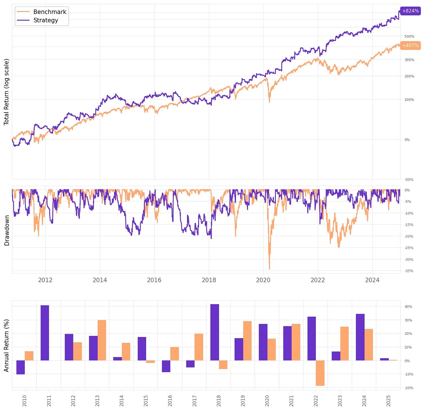
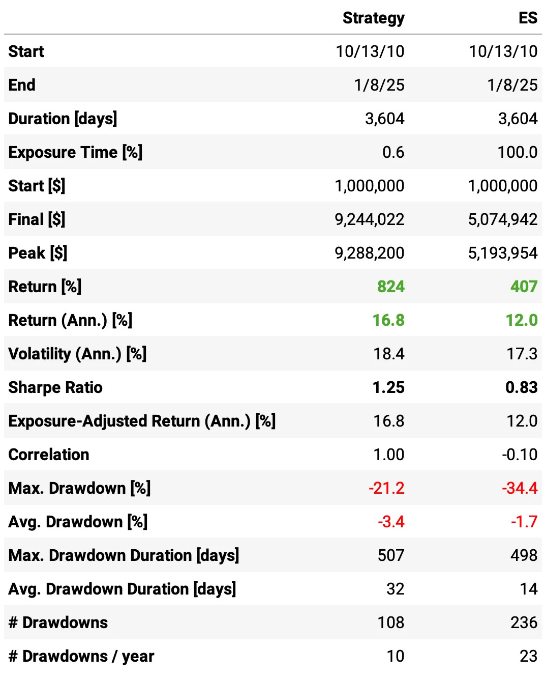
These changes produce the following results:
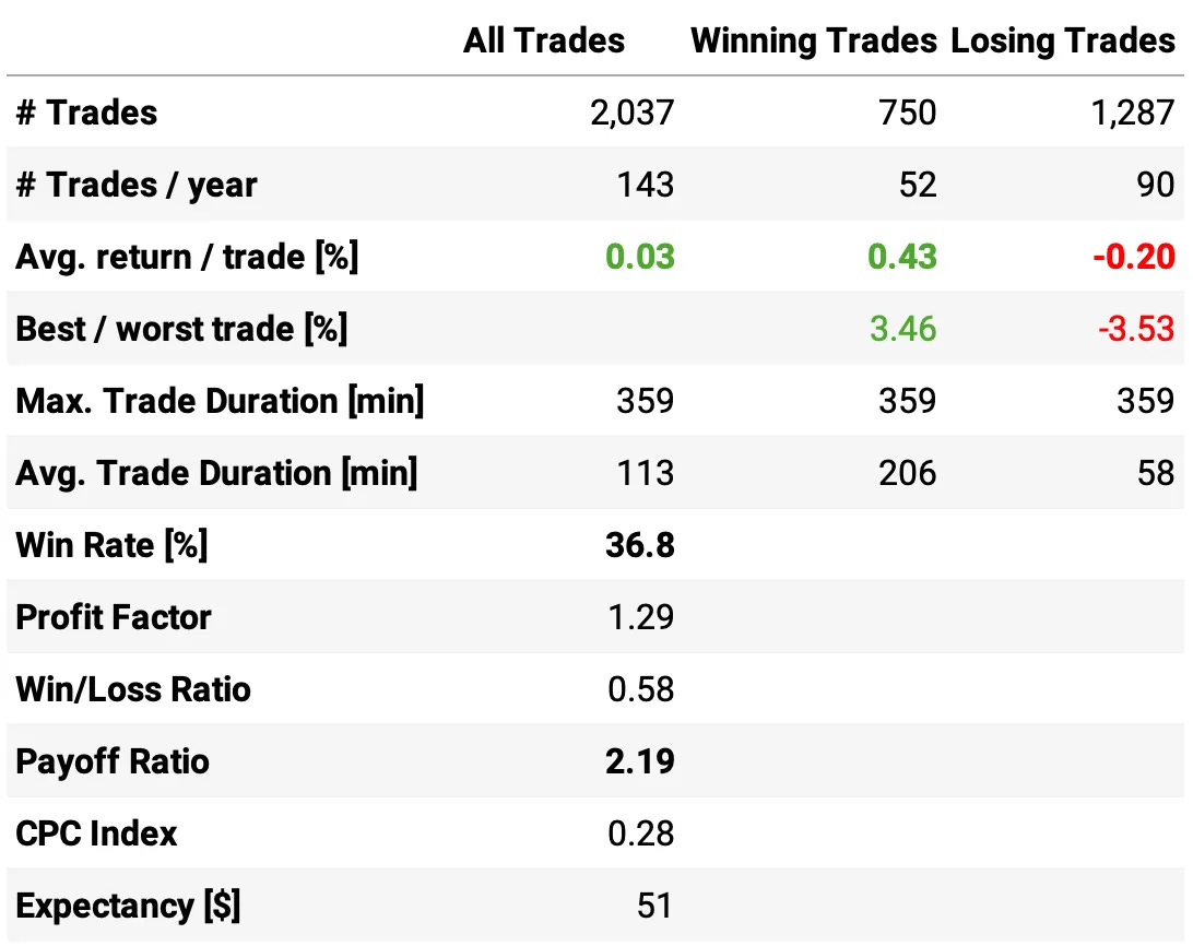
The adjustments resulted in a good improvement:
Annual returns more than doubled, now reaching 16.8% vs. 12% the benchmark;
Sharpe ratio increased from 0.91 to 1.25;
Max drawdown reduced from 24% to 21%;
All trade statistics improved.
What else can we do to improve the results further?
Diversification
My first idea when I initially read the paper was to apply the strategy across a basket of stocks, such as S&P 500 or Nasdaq-100 constituents, and trade multiple stocks simultaneously, thus taking the advantage of automation. However, I couldn't make such a system work.
For some stocks (like the ones shown in the end of the paper), the model does work. Unfortunately, according to my tests, this is not true for most of the stocks in a larger basket. And cherry-picking stocks after seeing their backtest results is the text-book definition of selection bias.
So, to add some diversification, I decided to consider only two instruments: ES and NQ, the two most liquid futures contracts in stock indices.
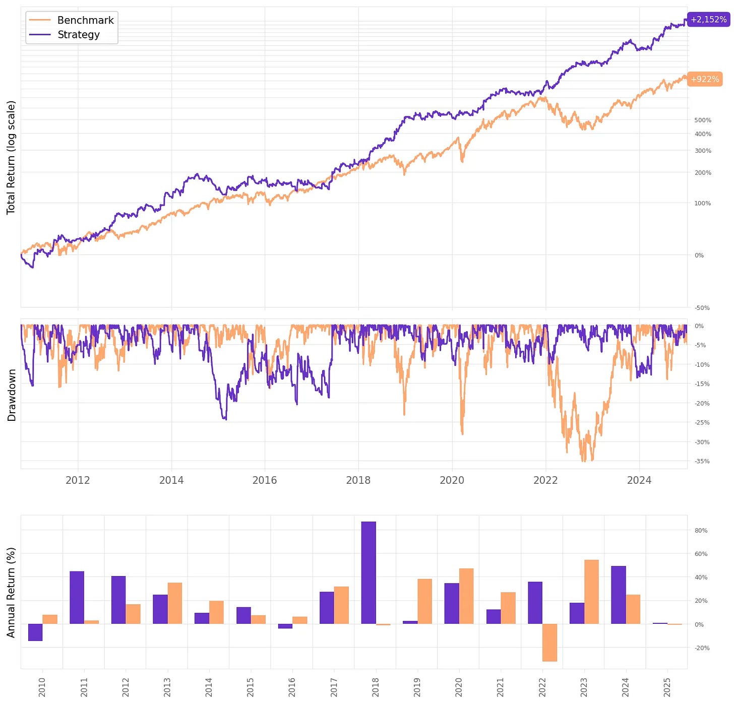
First, let's see how the model performs when applied to NQ:
The system works well on NQ as well:
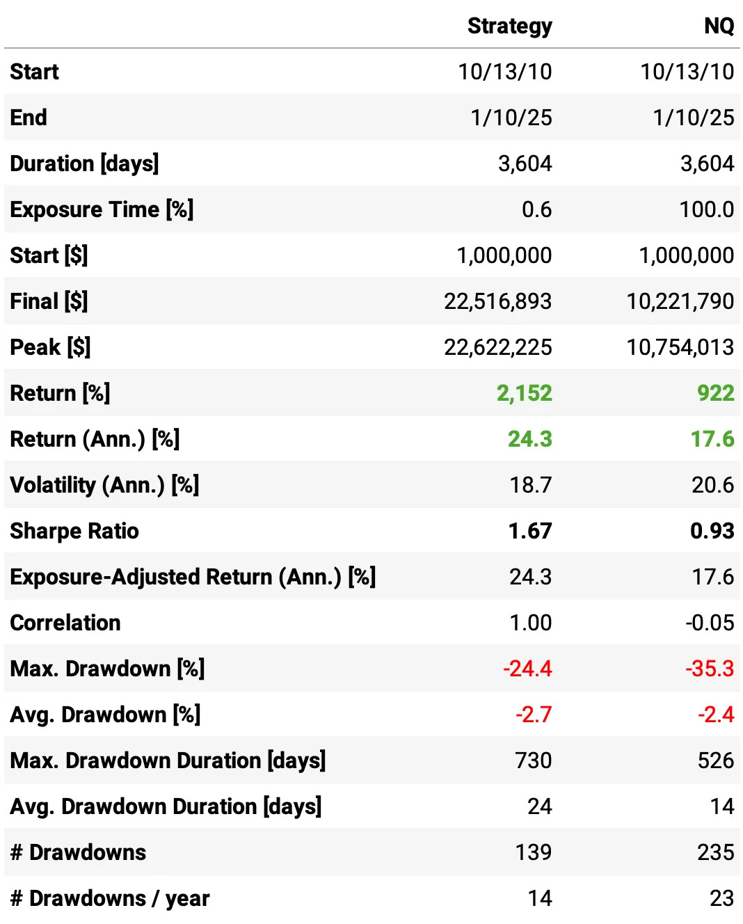
Annual return is at 24.3% vs. 17.6% the benchmark;
Sharpe ratio achieves 1.67 vs. 0.93 NQ long only;
Max drawdown is at 24% vs. 35% the benchmark;
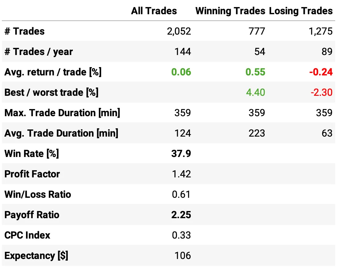
The expected return per trade is +6 bps, with a win ratio of 38% and a payoff ratio of 2.25.
Now, we create a portfolio allocating our capital with the following weights:
50% on the strategy applied to NQ;
25% on strategy applied to ES;
25% on NQ long only.
The weights that maximize the Sharpe ratio would be 45%, 15% and 40% - but that would be too much optimization to my taste.
So, these are the results for the portfolio:
Highlights:
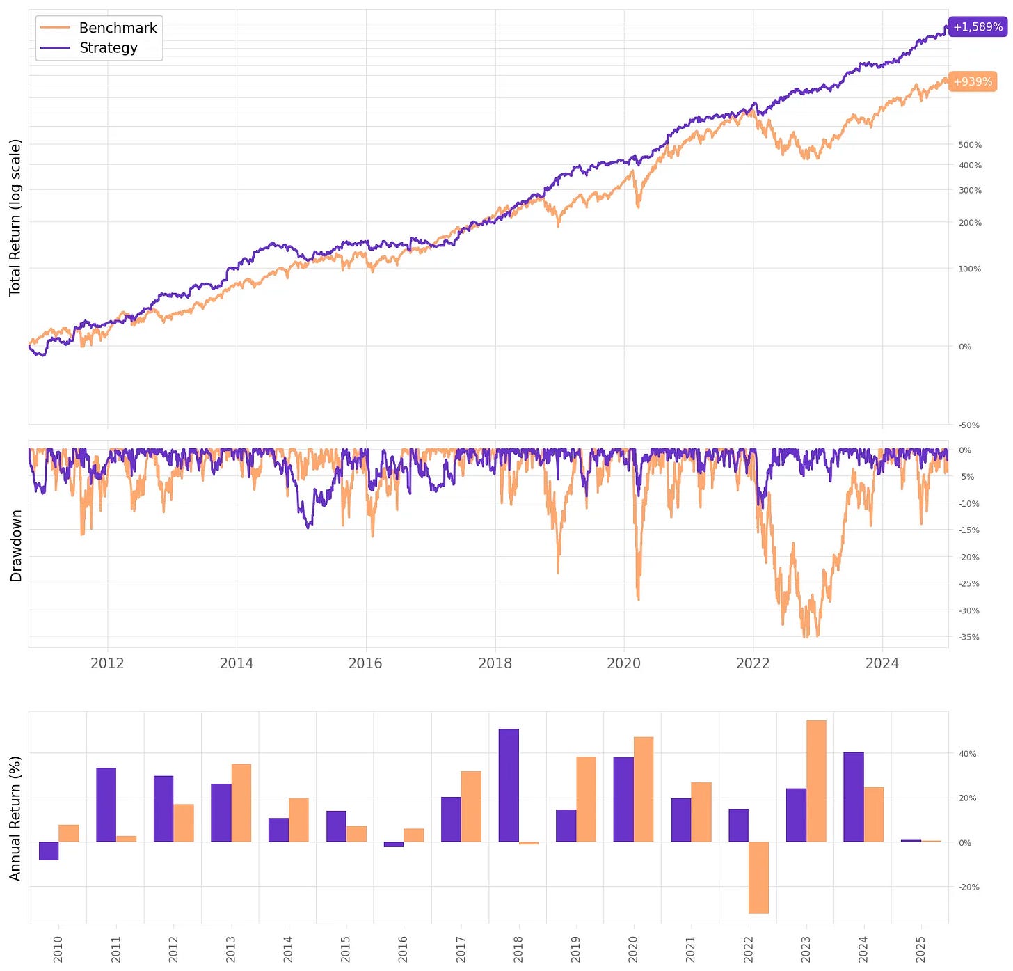
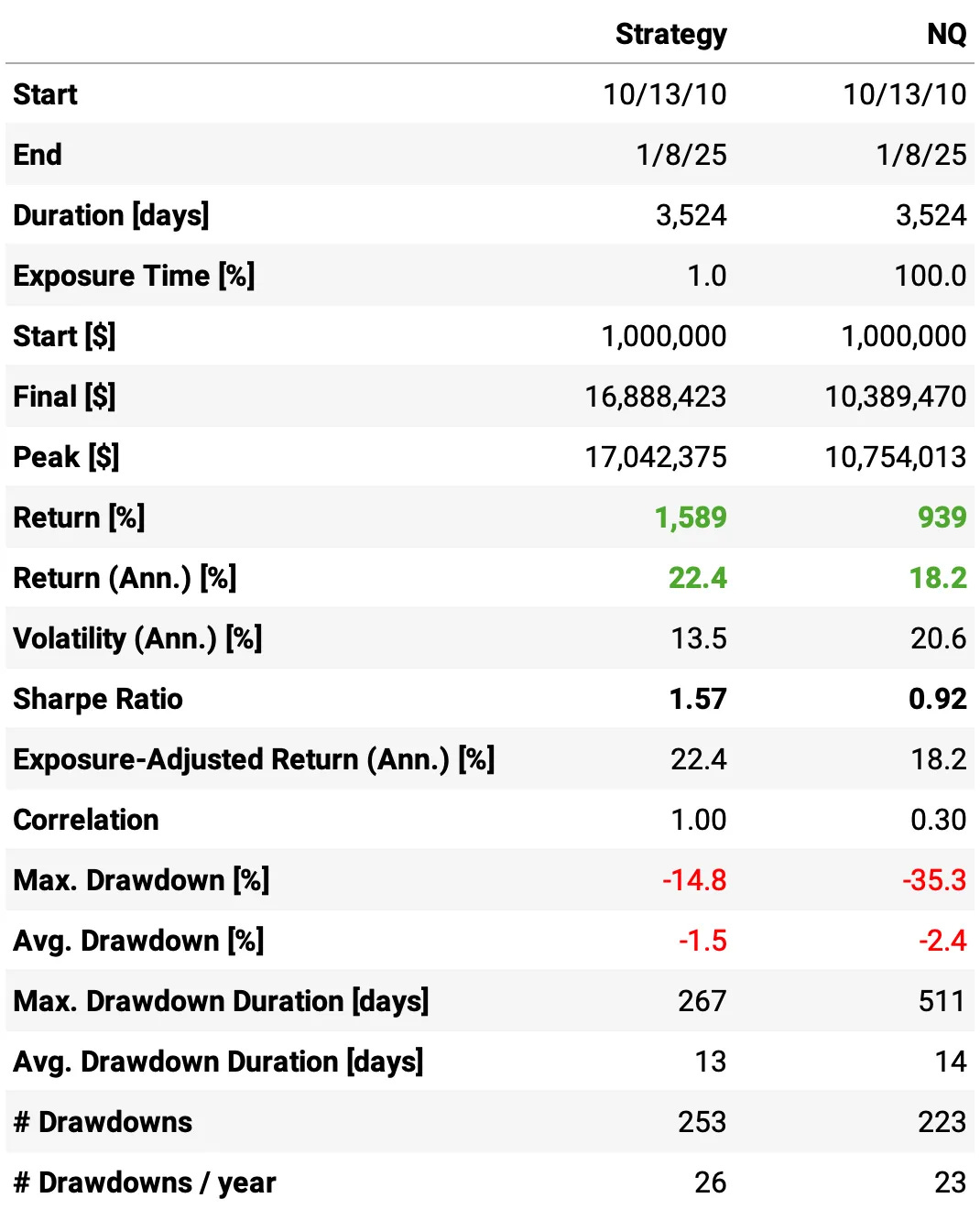
Annual returns reaches 22.4% vs. 18.2% benchmark;
Sharpe ratio is now at 1.57 vs. 0.92 NQ long only;
Maximum drawdown is 15%, less than half of the benchmark's
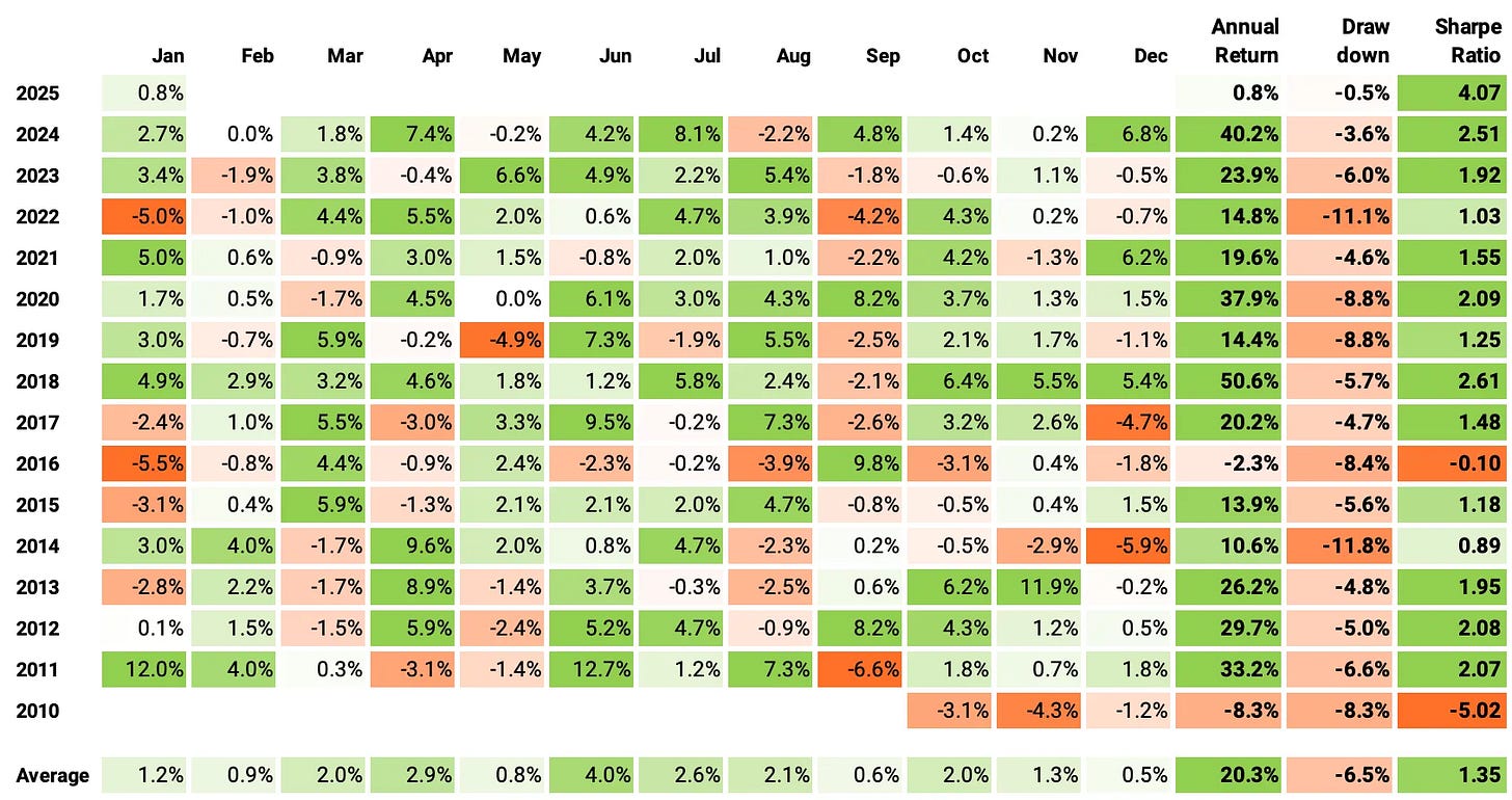
Now, let's see the monthly and annual returns:
If we had traded this strategy since 2010:
We would have had 2 negative years in 16;
We would have seen 65% of the months positive, with the best at +12.7% (Jun'11);
We would have seen 35% of the months negative, with the worst at -6.6% (Sep'11);
The longest positive streak would have been 11 months, from Apr'20 to Feb'11;
The longest negative streak would have been 4 months, from Oct'14 to Jan'15.
Final thoughts
Over the past several weeks, I've spent a lot of time implementing and deploying strategies live. As the number of live systems and the AUM increase, continuing to write and share ideas is getting harder. But I am committed to continue.
I am definitely forward-testing this system; if the forward-test results come in line with the backtest, this model will be a great addition to the portfolio.
I'd love to hear your thoughts about this approach. If you have any questions or comments, just reach out via Twitter or email.
Cheers!




Thanks for writing this. Interesting and elegant! I am curious if there are other methods like this that are "simple" and elegant. I have couple of thoughts:
1. As an example, if the price goes above noise area, and then comes back to the vwap/noise area where it is closed. Is another trade not opened until it crossed the opposite noise area? Or can the trade be opened on the same side the first trade was taken and closed?
2. Instead of having a trade at half hourly intervals to reduce premature closing/opening of trades. Would something like Kaufman moving average be used, and then it doesn't need to be at half hour intervals?
I have been working on replicating the result of your NQ futures version but I found my results are quite deviating and I think I have done something wrong. May I ask in your version do you ignore the trade starting at 09:30:00? My trades numbers have gone to around 10085 trades.