Fast trend following

+20% annual returns with a trend-following system in a shorter timeframe

Richard Dennis, Chicago's trading legend who famously turned a $1,600 loan into a $200 million fortune

The idea

“I always say that you could publish trading rules in the newspaper and no one would follow them. The key is consistency and discipline.” Richard Dennis.

Richard Dennis is one of the greatest trend-following traders in history, renowned for transforming a small loan into a fortune in the commodities markets. As a pioneer of systematic trading, Dennis believed that successful trading could be taught, leading to the famous Turtle Traders experiment in the 1980s. In this bold experiment, he trained a group of novices to follow a simple trend-following system, proving that discipline and consistency, not innate talent, were the keys to trading success.

This week, let's view a trend-following idea applied to the futures market. This article will be similar to A Mean Reversion Strategy from First Principles Thinking; let's follow a similar approach. Here's our plan:

1. First, we will deconstruct a trend-following strategy into its basic components;

2. Then, we will propose a new way to identify when a trend starts and ends;

3. Next, we will devise a strategy based on this new indicator and run some experiments;

4. Finally, we will discuss how to improve further.

Deconstructing a trend following strategy

Let's break down a trend-following strategy into smaller, more manageable parts:

• Entry trigger. Every trend-following strategy has a set of entry rules that, when triggered, tell us to go long (or short) if the instrument's price has started to trend up (or down). Typically, these entry rules are based on price movements breaking above or below predefined thresholds, such as moving averages, channel breakouts, or volatility bands. For example, an entry might be triggered when the price closes above a long-term moving average or surpasses a recent high.

• Exit trigger. Also, every trend-following strategy has a set of exit rules that, when triggered, tell us to close the position. They try to signal the trend started to reverse. These exit rules often rely on trailing stops, such as moving averages, recent lows (for long positions), or volatility-based stops. The goal is to allow the strategy to ride the trend as long as it persists while minimizing losses when it ends. This ensures the strategy captures large price moves while managing downside risk.

Our strategy will focus on NQ futures (always the most liquid contract), with a 1-minute timeframe. The simplest possible choice would be to define entry and exit triggers with moving averages. As I am an engineer, I prefer Kalman filters. They offer some advantages over moving averages:

• Noise Reduction: Kalman filters are highly effective at reducing noise in price data, providing smoother signals for identifying trends compared to traditional moving averages.

• Adaptability: Unlike fixed moving averages, Kalman filters dynamically adjust to changing market conditions, making them more responsive to trend shifts.

• Robustness: They incorporate both historical data and statistical models, improving their ability to predict trends and filter out false signals.

• Efficiency: Kalman filters can provide a clearer signal with fewer lagging effects, allowing for more timely entries and exits in rapidly changing markets.

• Flexibility: They can be customized to suit different trading timeframes and objectives, offering a more tailored approach to trend-following strategies.

NQ 1-minute closing prices on March 8th, 2022, with two Kalman Filters

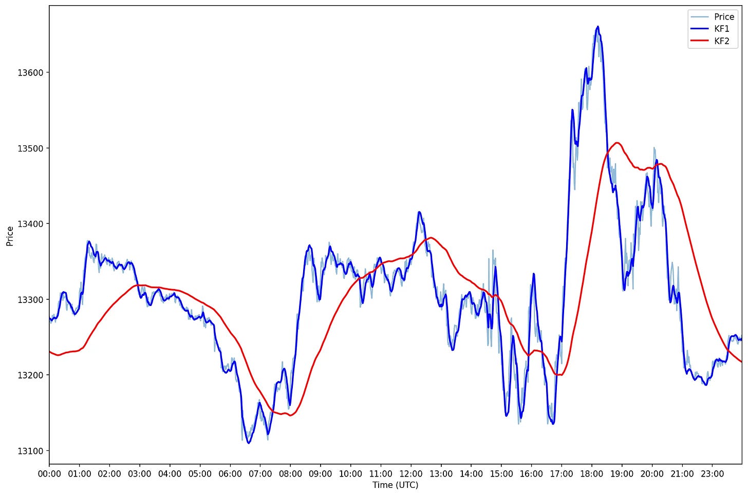
The chart above shows the price of NQ in light blue on a given day and two Kalman filters - one in dark blue and one in red. To explain the difference between them, let me briefly explain what is a Kalman filter.

A Kalman Filter is an algorithm for estimating the state of a dynamic system. It combines noisy observations with predictions based on a mathematical model. The filter is widely used in control systems, robotics, and financial markets to filter noise from data and make more accurate predictions.

In financial markets, the Kalman Filter is particularly useful for smoothing price data, estimating trends, and identifying underlying patterns in the presence of market noise.

Key Components of the Kalman Filter

1. State Variables:

   • Represent the system being estimated. In this case:

     • price: The observed asset price.

     • trend: The estimated rate of change in the price.

2. Measurement:

   • Observations used to update the state. Here, the observed price (close) is the only measurement.

3. State Transition Matrix (F):

   • Defines how the state evolves over time:

     • new price = current price + trend

     • new trend = current trend

4. Measurement Function (H):

   • Relates the observed measurement (price) to the state:

     • observed price = true price (state variable)

5. Covariances:

   • Process Noise (Q):

     • Represents the uncertainty in the model's predictions.

   • Measurement Noise (R):

     • Represents the uncertainty in the observed data.

6. Uncertainty (P):

   • Represents the initial uncertainty about the system's state.

Impact of the Noise Parameter (R)

The measurement noise (R) is a critical parameter in the Kalman Filter, and its value influences how the filter balances trust between the model's predictions and the observed data.

1. Low R (Low Measurement Noise - the dark blue line):

   • The filter assumes the observations are highly reliable.

   • The estimate closely follows the observed data, reacting quickly to changes in the measurements.

   • Impact: May result in overfitting to noisy data, reducing smoothness.

2. High R (High Measurement Noise - the red line):

   • The filter assumes the observations are noisy and unreliable.

   • The estimate relies more on the model's predictions, leading to smoother output.

   • Impact: May lag behind sudden changes in the data (e.g., sharp trend reversals).

My idea is not to provide a full review of Kalman filters. I believe, though, this brief introduction is enough to give anyone the basics so we can move forward to our next step.

The QT indicator

Looking at the previous chart, we observe the blue line is always oscillating above and below the red line. So, we can compute the percentage difference between the blue line and the red line - which will be positive if the blue line is above the red line, or negative otherwise.

If we were to plot these percentage differences in a histogram, we would see a nice Gaussian curve (with fatter tails to make Nassim Taleb happy :)).

But instead, let's compute the percentiles for each of these differences, such that:

• +100 will be the highest difference % in our distribution (the positive value farthest from the red line);

• -100 will be the lowest difference % in our distribution (the negative value farthest from the red line);

• 0 will be mid value (exactly on top of the red line).

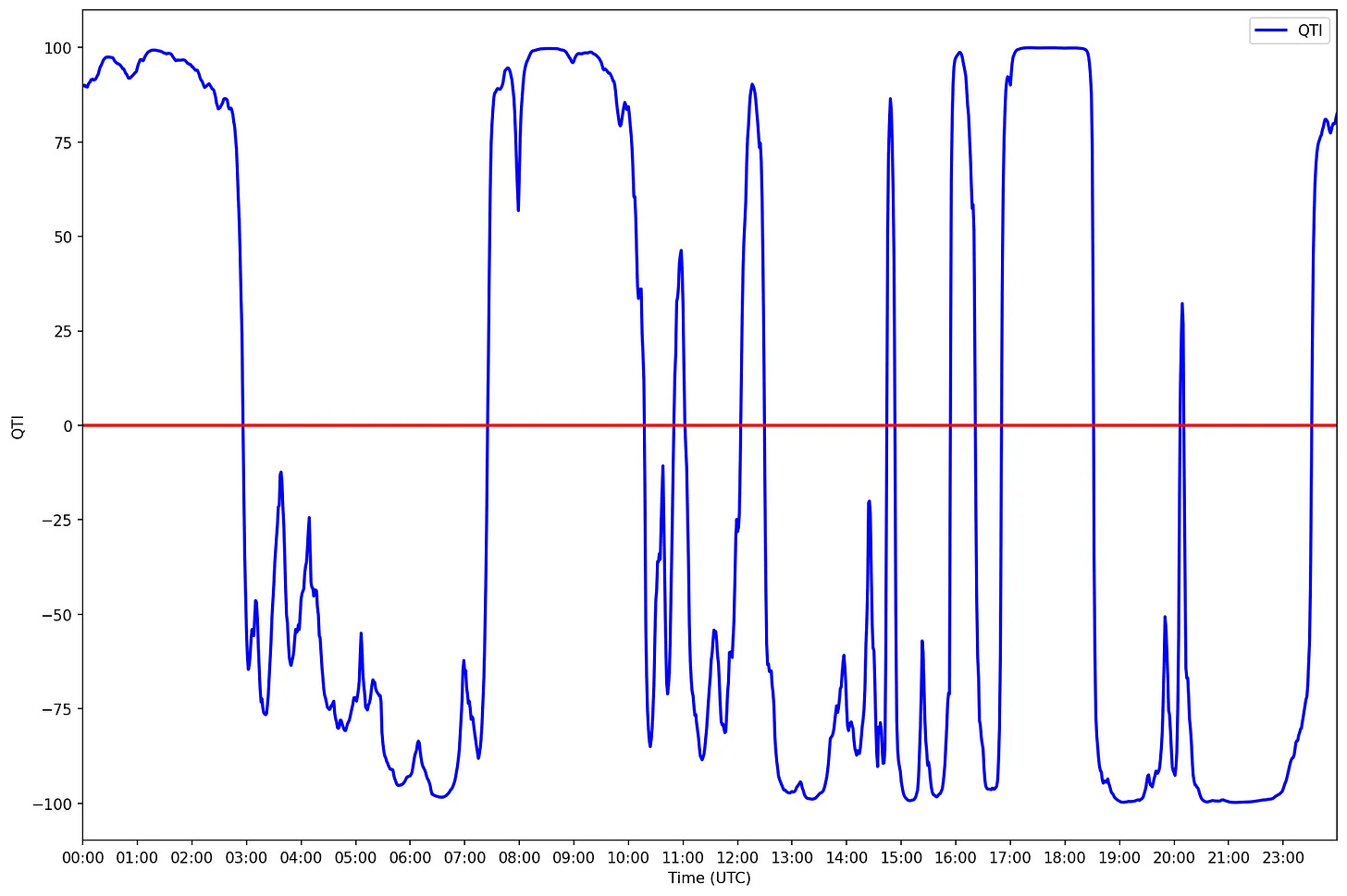
Now, if we plot these values for a given day, that would be like if we took the both ends of the red line and pulled it, straightening it:

NQ 1-minute Quantitativo Trend Indicator on March 8th, 2022

For the lack of a better name, let's call this indicator QTI (Quantitativo Trend Indicator). It indicates how far the (smoothed) prices (the blue line) are from the trend (the red line):

• +100 means the price is well above the trend;

• -100 means the price is well below the trend;

• 0 means the price is exactly on the trend line;

• If the indicator is crossing above the red line up, this means the price is trending up;

• If the indicator is crossing below the red line down, this means the price is trending down.

Now, let's devise a strategy using this indicator.

The strategy

Our strategy will be either 100% long, 100% short, or out of the market. Here's how we will determine our position:

• Whenever NQ's QTI crosses above 5, we will open a long position, set a profit target at QTI 35, and stop loss at 5;

• Whenever NQ's QTI crosses below -90, we will open a short position, set a profit target at QTI -95, and a stop loss at -90.

That's it. Let's run some experiments.

Experiments

This week's strategy is a bit different than what I've been writing so far in some important aspects. So, here are the assumptions on the experiments:

• Trading around the clock. This strategy trades 1-minute bars (data from Databento) starting mid-2017. So, we will assume trading whenever NQ is trading. We will trade at the closing prices of the 1-minute bars.

• No compounding. Throughout the experiments, we will trade only a single contract. We will be either long this 1 contract, short this 1 contract, or out of the market.

• Leverage. Trading futures allow us to use leverage. We will use 4x leverage by having our starting capital as 1/4 of the notional value of 1 contract.

• Trading costs. NQ is one of the most liquid contracts there is (we will always trade the front month contract). The bid-ask spread really tight, usually 1 tick or 0.25 index points. This means the bid-ask spread is ~1/10th of a basis point. So, in these experiments, we will not consider slippage nor commission (which can be easily added later; IBKR for example charges $0.85/contract).

Let's see how our first experiment fares:

Equity and drawdown curves for the first experiment

Summary of the backtest statistics

Summary of the backtest trades

Highlights:

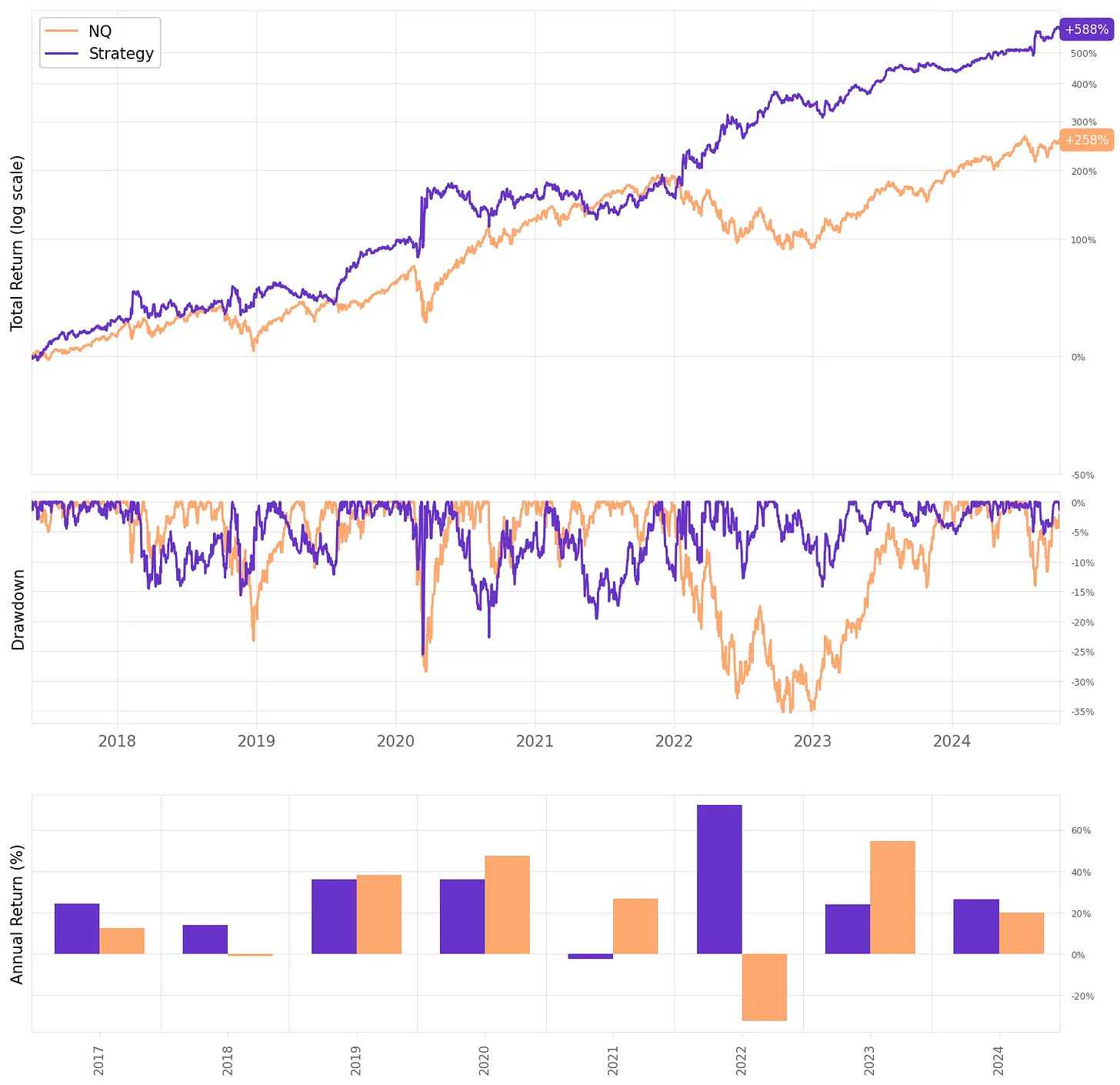
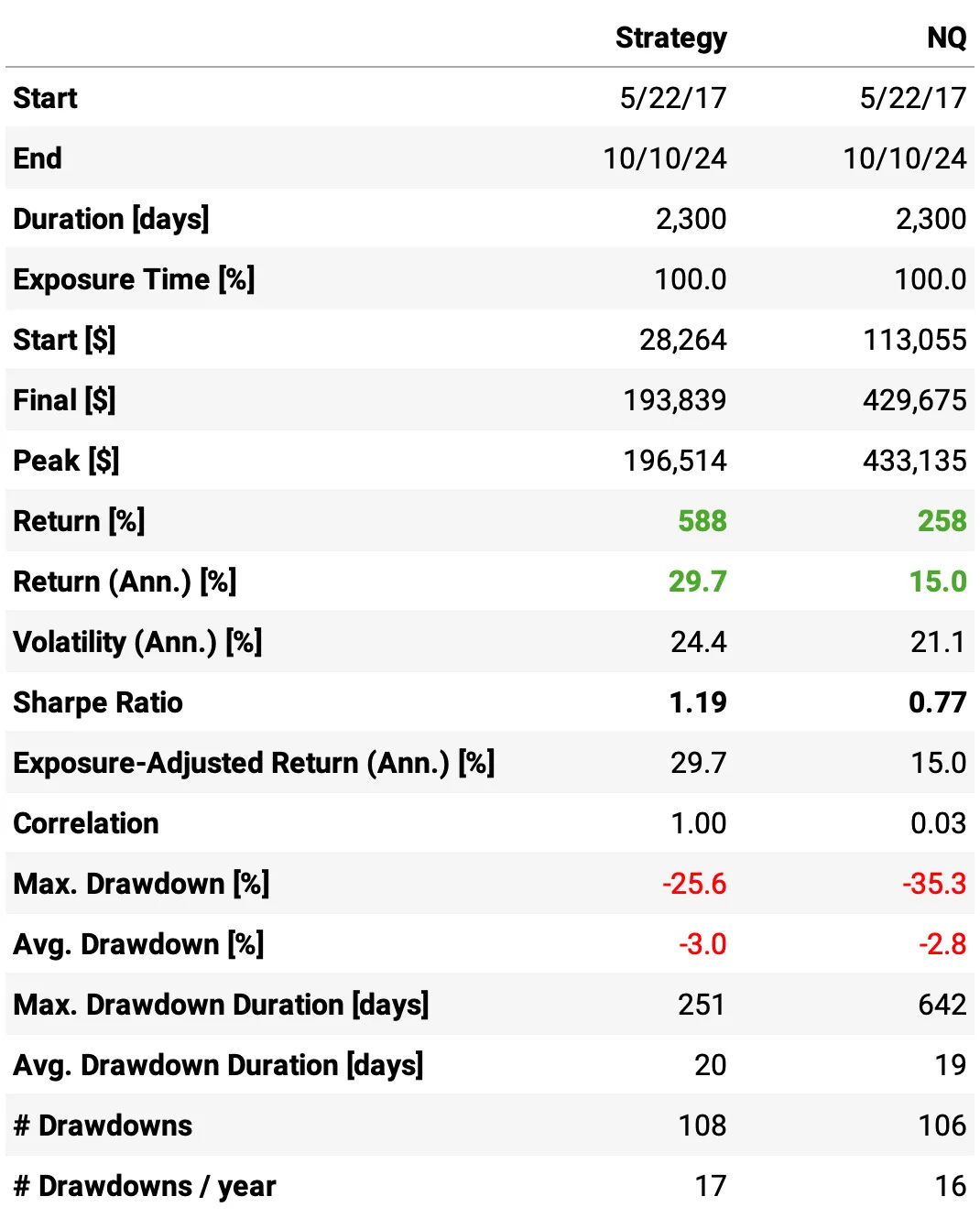
• The annual return achieved is 29.7% vs. 15.0% the NQ in the same period;

• The strategy was positive in all years except 2021 (near zero);

• The maximum drawdown is at 26%, vs. 35% the benchmark;

• The risk-adjusted return is at 1.19 (Sharpe), vs 0.77 the benchmark;

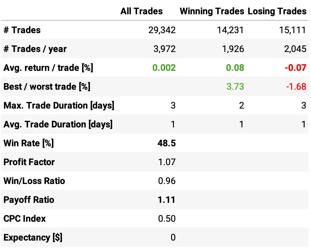
• The strategy trades 3,972 times/year, or about 16 times/day, with a win rate of 48.5%, profit factor of 1.07 and payoff ratio of 1.11;

How to improve this strategy?

Choosing parameters to entry and exit

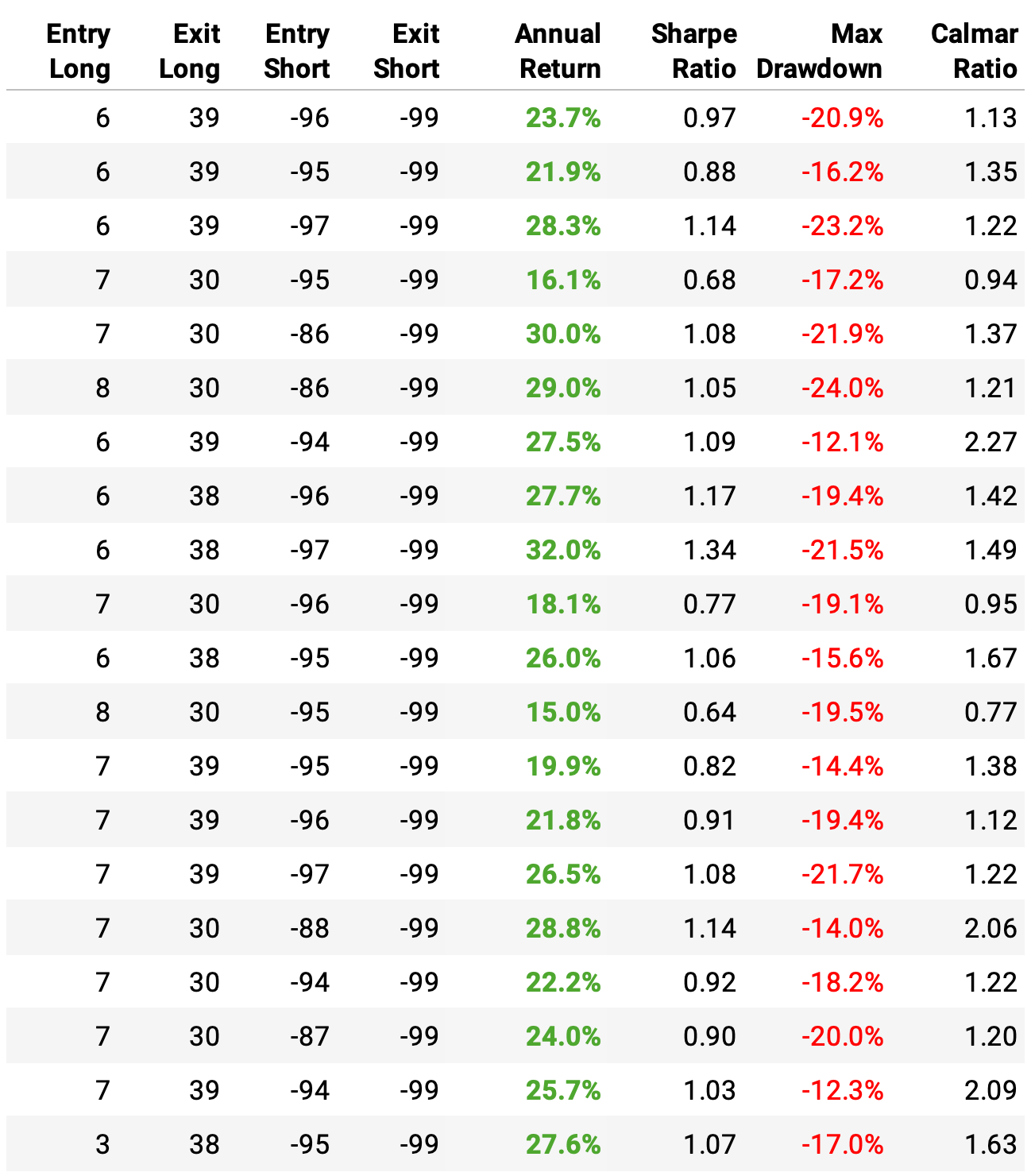
The entry and exit parameters used in the first experiment were arbitrarily chosen. Let's search for optimal parameters:

• We will search for the best combination of parameters varying the entries and exits in terms of QTI around 1-10, 30-40 for longs, and (85)-(97), (87)-(99) for shorts;

• The in-sample period will be from 2017 until the end of 2021, where we will perform the search;

• The out-of-sample period will be from 2022 on.

Running the search, here's what we find out of sample:

Out-of-sample results of the in-sample best parameters

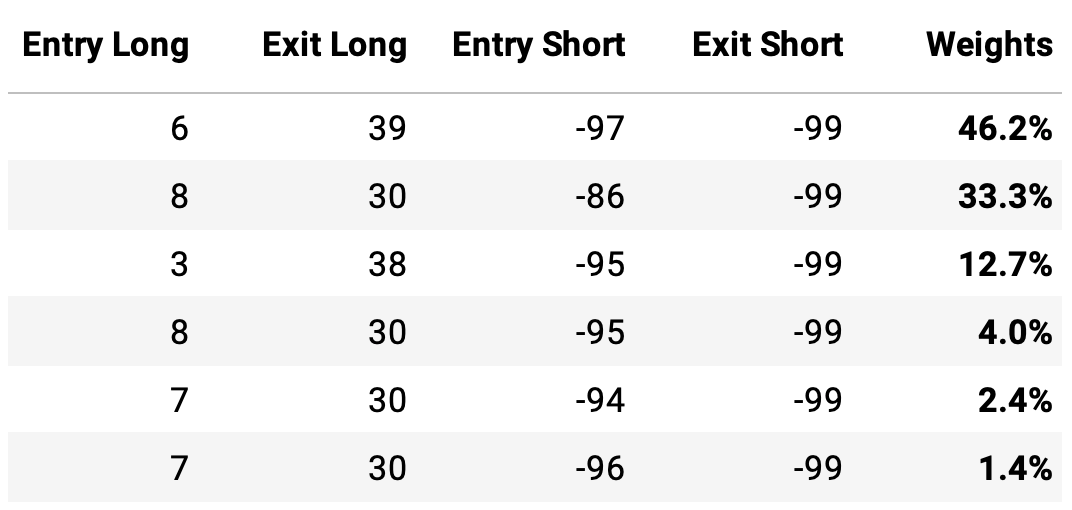
Now, instead of cherry-picking one of these sets of parameters, or simply averaging them out, let's assemble a portfolio with the 10 sets of parameters. To determine the weights, let's run a simple optimization algorithm on the in-sample daily returns, with the objective of maximizing the Sharpe ratio. Then, we can apply these weights to the out-of-sample period.

The weight results from the optimization on the in-sample period are:

In-sample weights of the optimization (target: Sharpe ratio)

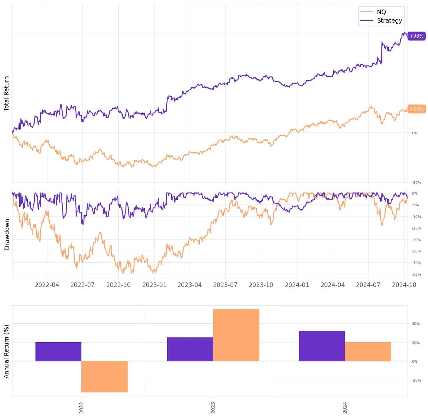
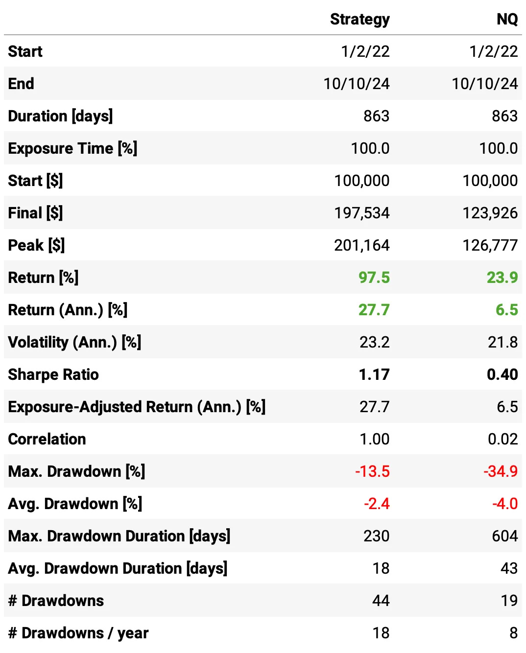
These are the results for the optimized portfolio out-of-sample:

Equity and drawdown curves for the optimized portfolio

Summary of the backtest statistics out-of-sample

Highlights:

• The annual return reached 27.7% vs. 6.5% the NQ in the same period (since Jan'22);

• The maximum drawdown is at 13.5% vs. 35% the benchmark;

• Sharpe ratio is at 1.17 vs. 0.40 NQ.

Now, let's look at the monthly and annual returns out-of-sample:

Monthly and annual returns

If we had traded this strategy since 2022:

• We would have had only positive years;

• We would have seen 76% of the months positive, with the best at +11.2% (Feb'23);

• We would have seen 24% of the months negative, with the worst at -8.5% (Jun'22);

• The longest positive streak would have been 6 months, from Apr'24 to Sep'24;

• We would nave not seen two consecutive negative months.

Final thoughts

Several people have asked me to develop trend-following strategies, especially applied to futures. This is a first study in the trend-following/futures direction. I combined it with my curiosity in exploring shorter timeframes and Databento's datasets. But there's still much to do in that front.

In my experience, whenever we try shorter timeframes, we encounter challenges in the execution front. So, before trading a system like this, I would have to carefully develop the execution algorithm and observe it for a while until acquiring enough conviction that the forward test results were inline with the backtest results.

Here are some improvements and tests to run on this idea before moving into production:

• Diversify the system, applying it to several futures markets;

• Test it with different timeframes (5’, 10’, 15’, 30’, 1h, etc);

• Try more sets of noise parameters in the Kalman filters.

Over the past few months, I've been completely immersed in deploying and running live strategies. In November, we had a nice +8% return with all strategies combined. Looking forward, I believe I will be able to resume writing once a week or once every other week in January.

I'd love to hear your thoughts about this approach. If you have any questions or comments, just reach out via Twitter or email.

Cheers!