Coding Trend Factor

From Paper to Python: Implementing a High-Performing Factor from Academic Research

The idea

"Every great developer you know got there by solving problems they were unqualified to solve until they actually did it." — Patrick McKenzie.

Patrick McKenzie is a well-known software developer, entrepreneur, and writer, widely recognized for his work in the software industry, particularly in bootstrapped startups and software-as-a-service (SaaS) businesses.

He built his entire career around sharing everything he learned, and his blog posts and tweets are often cited as must-reads for software entrepreneurs.

His quote about developers solving problems for which they were initially unqualified reflects a fundamental truth in programming—many great developers learn by doing rather than waiting until they are "ready.”

This week, I will share the implementation of the paper "A Trend Factor: Any Economic Gains from Using Information Over Investment Horizons?" from Yufeng Han, Guofu Zhou, and Yingzi Zhu. This paper was published in the Journal of Financial Economics (2016).

Before we dive into the paper's code, let me share a bit about the why and the how. The why is basically two reasons. First, I love implementing papers. I think by coding classic ideas, new ideas can emerge. Second, I believe these implementations might help other people who like studying. After all, sharing code implementations is the #1 ask I have received from the +3,500 readers in these past 8 months.

Now, to the how. I will share paper implementations and suggestions I find interesting. Every week, I receive many suggestions. And I read a lot of papers. The code I share here will be written in Python. I also like to code in C++, but I believe Python is more suitable for what I intend to write. I plan to share some implementations for free (like this one); I intend to put others on a larger course I want to launch. More on that later.

Finally, I love how the Gitbook platform works: it's great for creating and sharing code documentation and looks beautiful. In particular, I believe they do a much better job as a code-sharing platform than Substack. Therefore, I will share the implementations on both platforms: here and Gitbook. If you are like me, you'll prefer Gitbook.

Why implement this paper?

The idea to write about this paper first appeared when I read another paper: “Design Choices, Machine Learning, and the Cross-section of Stock Returns” by Minghui Chen, Matthias X. Hanauer, and Tobias Kalsbach. The suggestion to read this came from one of

QuantSeeker

's great weekly recaps.

There, I found this table on page 33:

The most important features, according to the paper

Figure 6 also illustrates the same point:

The most important features, according to the paper

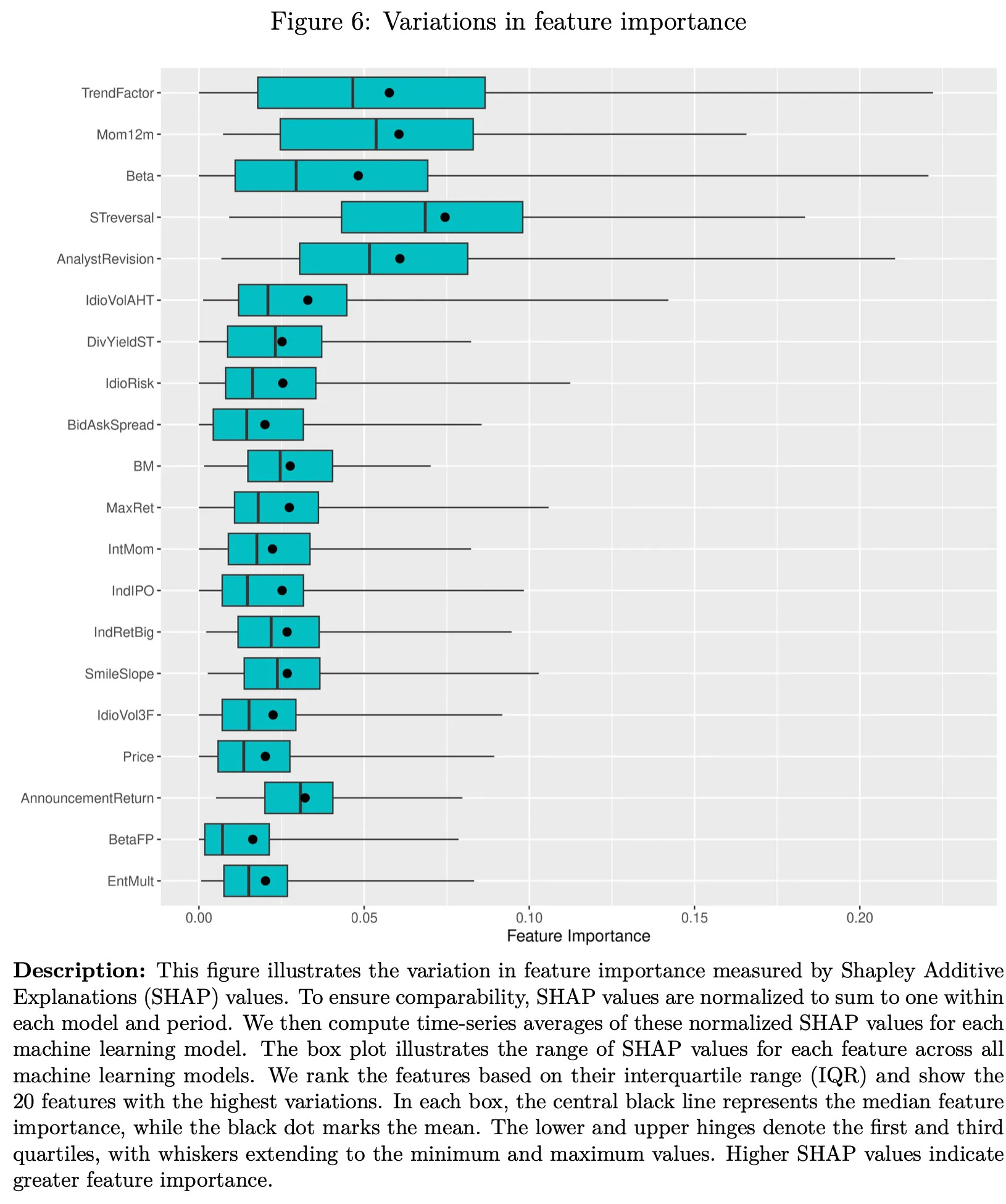
The table and the chart showed this TrendFactor feature as one of the most important predictors in the model. Looking at the references, I discovered that this feature was introduced in the paper "A Trend Factor: Any Economic Gains from Using Information Over Investment Horizons?" by Yufeng Han, Guofu Zhou, and Yingzi Zhu, published in the Journal of Financial Economics (2016).

Unlike previous studies that examine short-term reversals (daily/monthly), momentum (6-12 months), and long-term reversals (3-5 years) separately, the authors construct a single factor that incorporates all three price trends using moving averages over different time horizons.

In the paper, the authors report that the trend factor earns an average return of 1.63% per month, significantly higher than short-term reversal (0.79%), momentum (0.79%), and long-term reversal (0.34%). It more than doubles the Sharpe ratios of existing factors.

During the 2007-2009 financial crisis, the trend factor earned +0.75% per month, while:

• The market lost -2.03% per month.

• The momentum factor lost -3.88% per month.

• The short-term reversal factor lost -0.82% per month.

• The long-term reversal factor barely gained 0.03%.

Let's dive into the implementation. You can continue reading here or head to Gitbook for a better reading experience.

Data

The study uses daily stock prices from January 2, 1926, to December 31, 2014, obtained from the Center for Research in Security Prices (CRSP).

Our replication will use daily stock prices from January 1, 1990, to January 1, 2025, obtained from Norgate data. Norgate provides high-quality survivorship bias-free daily data for the US stock market that is very affordable. For more information on how to acquire a Norgate data subscription, please check the Norgate website.

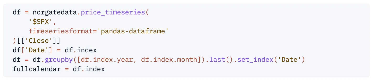
The paper explains that to compute the trend factor, monthly moving average signals are calculated at the end of each month. So, first, let's create a fullcalendar variable, which is a Pandas DatetimeIndex that holds the last trading day of each month:

Now, let's see what the paper says about the stock universe:

• The dataset includes all domestic common stocks listed on NYSE, AMEX and NASDAQ;

• The dataset excludes Close-end funds, REITs, unit trusts, ADRs and foreign stocks;

• Price Filter: Stocks with prices below $5 at the end of each month are excluded;

• Size Filter: Stocks in the smallest decile (based on NYSE breakpoints) are excluded.

These filters are applied to reduce noise and ensure liquidity, following the methodology used in Jegadeesh & Titman (1993) for constructing momentum strategies.

We will implement something close: we will only consider Russell 3000 current & past constituents. That should address the first, second, and last bullets above. Considering stocks only when they were part of the index also ensures we are not adding survivorship bias. Finally, we will exclude stocks whenever their unadjusted closing price is below $5. Here's how that translates into code for a given symbol:

Now, let's compute the moving averages (trend signals). Moving averages are computed at the end of each month using stock prices over different lag lengths. The moving average (MA) for stock j with lag L at month t is defined as:

\(A_{j,t,L} = \frac{P_{j,d-L+1} + P_{j,d-L+2} + \dots + P_{j,d}}{L}\)

where $P_{j,d}$ (I know, this is not good… but Substack does not support inline LaTex… but Gitbook does, check it out) is the closing price for stock j on the last trading day d of month t, and L is the lag length. Then, we normalize the moving average prices by the closing price on the last trading day of the month:

\(\tilde{A}_{j,t,L} = \frac{A_{j,t,L}}{P_{j,d}}\)

This ensures stationarity and prevents biases from high-priced stocks.

The paper considers MAs of lag lengths 3-, 5-, 10-, 20-, 50-, 100-, 200-, 400-, 600-, 800- and 1,000-days. Let's see how this translates into code:

We are getting to the final steps of the data-gathering stage. Now, we must add the target variable that will be used to predict the monthly expected stock returns cross-sectionally.

In other words, we must compute the next month return for every date:

1. First, we gather the prices from a given symbol;

2. Next, we compute the normalized MAs for all lags;

3. Then, we select only the last day of every month and compute the next month's return;

4. Finally, we apply the size/price filters.

We already did (1), (2) and (4). Now, let's see how to do (3):

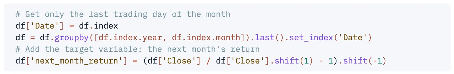
It's important to observe the correct use of the .shift(x) operator.

.shift(1) gets the previous value, while .shift(-1) gets the next value. Messing with these operators is a common source of error in many quant codebases found online.

So, when we run (df['Close'] / df['Close'].shift(1) - 1) , we are computing the current month's return. After that, when we apply .shift(-1) , this results in the next month's return, which is exactly what we need.

Now, let's put everything together into a method that retrieves data for a given symbol:

The last few lines organize the columns and the index. The index, in particular, is organized in a Multi-level indexing, which is a great Pandas feature to work with higher dimensional data. To more information about MultiIndex / advanced indexing, please check Pandas documentation.

Let's see the data from the past 12 months of AAPL by running get_data('AAPL').tail(12) :

Data from the past 12 months of AAPL

We can now gather data for all stocks in the Russell 3000 universe:

The data DataFrame is a table with approximately 800k rows and 12 columns that looks like this:

DataFrame ready to compute the trend factors

Great! We are ready to move to the next step: compute the trend factors. It's important to highlight how the data is organized:

• In the first level of our index, we have the last day of each month;

• In the second level of our index, we have all stocks in our universe for that particular date;

• In the columns, we have the MAs computed with the prices up until that specific date for that specific stock, and the next month return for that particular stock.

Step 1: Cross-sectional regressions

To predict the monthly expected stock returns cross-sectionally, we use a two-step procedure. In the first step, we run in each month tt a cross-section regression of stock returns on observed normalized MA signals to obtain the time-series of the coefficients on the signals:

\(r_{j,t} = \beta_{0,t} + \sum_{i} \beta_{i,t} \tilde{A}_{j,t-1,L_i} + \varepsilon_{j,t}\)

where:

• $r_{j,t}=$ return on stock j in month t

• $\tilde{A}_{j,t-1,L_i}=$ trend signal at the end of month t−1 on stock j with lag $L_i$

• $\beta_{i,t}=$ coefficient of the trend signal with lag $L_i$ in month t

• $\beta_{0,t}=$ intercept in month t

To do the regressions, we will use Python's Statsmodels package. We loop through all dates, doing the cross-sectional regressions:

The code above is straightforward. It produces the coefs DataFrame, a table with close to 400 rows and 12 columns with all \beta_{i,t} coefficients:

Coefficients of the trend signals

The paper has the following important sentence: "It should be noted that only information in month ttt or prior is used above to regress returns in month t." This is what the .shift(1) operator in the last line of the last code block is for. Omitting that code would result in lookahead bias and results too good to be true.

Step 2: Expected returns

We estimate the expected return for month t+1 from

\(E_t[r_{j,t+1}]=\sum_i E_t[\beta_{i,t+1}] \tilde{A}_{j,t,L_i}\)

where $E_t[r_{j,t+1}]$ is our forecasted expected return on stock j for month t+1 and $E_t[\beta_{i,t+1}]$ is the estimated expected coefficient of the trend signal with lag $L_i$ and is given by

\(E_t[\beta_{i,t+1}] = \frac{1}{12}\sum_{m=1}^{12} \beta_{i,t+1-m}\)

which is the average of the estimated loadings on the trend signals over the past 12 months.

First, let's compute the matrix $E_t[\beta_{i,t+1}]$:

Estimated expected coefficients of the trend signals

Note that we do not include an intercept above because it is the same for all stocks in the same cross-section regression, and thus it plays no role in ranking the stocks.

Trend factor

Now, we are ready to construct the trend factor. We loop through all dates, performing the dot product between the estimated expected coefficients of the trend signals and the trend signals matrices:

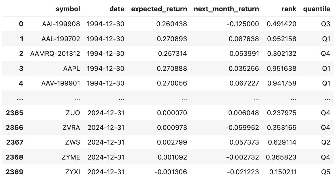
And that's all there is to it. We get the following table, with approximately 800k rows and 4 columns:

Trend factors for every symbol-date pair

In our last step, we sort all stocks into five portfolios by their expected returns. The portfolios are equal-weighted and rebalanced every month. The return difference between the quintile portfolio of the highest expected returns and the quintile portfolio of the lowest is defined as the return on the trend factor. Intuitively, the trend factor buys stocks that are forecasted to yield the highest expected returns (Buy High) and shorts stocks that are forecasted to yield the lowest expected returns (Sell Low).

Adding the quantiles is straightforward:

The code above produces the following table:

Trend factor quantiles

Now, we group by date:

The rets DataFrame has the monthly returns and the number of stocks from each quantile, as we can see below:

Final results

Visualizing the results

Finally, we can plot the return of the trend factor:

Looking at this equity curve, we see that the factor performs until 2016. After that, it's basically flat. If we reduce the exposure on the shorts to 0.5 instead of 1, we can get a better equity curve.

Adding a bit of formatting, we get the following:

TrendFactor equity curve

Summary of backtest statistics

We can also see the average return per quantile:

Returns for each quantile

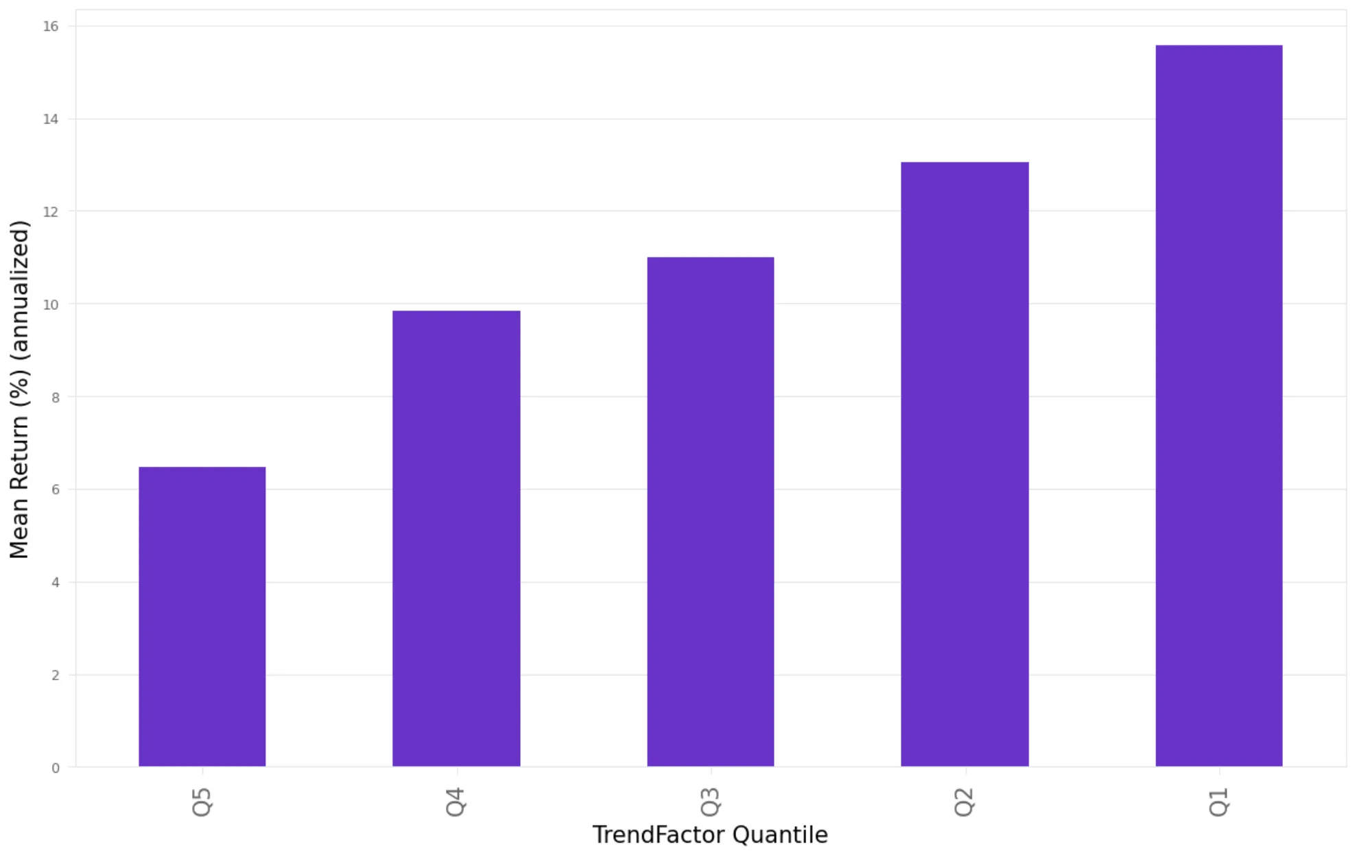
And finally, we can see the monthly and annual returns:

Monthly and annual returns

Conclusion

This paper introduces a trend factor that synthesizes short-, intermediate-, and long-term price trends using moving averages, significantly outperforming traditional factors like momentum, short-term reversal, and long-term reversal. The trend factor provides higher returns, better risk-adjusted performance, and reduced crash risk, making it a valuable addition to both asset pricing models and portfolio construction strategies.

Implementing this approach in Python is a good exercise in quantitative finance and systematic trading. It allows practitioners to explore data handling, time-series analysis, and cross-sectional regressions using libraries such as Pandas, NumPy, and Statsmodels. Coding this methodology in Python is a practical way to deepen one’s understanding of factor-based investing and trend-following strategies.

I'd love to hear your thoughts about this. If you have any questions or comments, just reach out via Twitter or email. Also, I would love if you could answer a few questions about the content I am sharing: this is useful in determining what to share in the next articles, and how:

Cheers!